Dead Reckonings

The previous Part I of this essay described the construction of straight-line nomograms using simple geometric relationships. Beyond this, a brief knowledge of determinants offers a powerful way of designing very elegant and sophisticated nomograms. A few basics of determinants are presented here that require no previous knowledge of them, and their use in the construction of straight line nomograms is demonstrated. Then we will see how these determinants can be manipulated to create extraordinary nomograms.

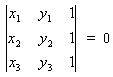
A matrix consists of functions or values arranged in rows and columns, as shown within the brackets in the figure on the right. The subscript pair refers to the row and column of a matrix element. A determinant represents a particular operation on a matrix, and it is denoted by vertical bars on the sides of the matrix. The determinant this 3×3 matrix is given by

a₁₁a₂₂a₃₃ + a₁₂a₂₃a₃₁ + a₁₃a₂₁a₃₂ – a₁₃a₂₂a₃₁ – a₁₁a₂₃a₃₂ – a₁₂a₂₁a₃₃

But there are visual ways of deriving it. In the first figure the first two columns of the determinant are repeated to the right of the original, and then the products of all terms on diagonals from upper left to lower right are added and the products of all terms on diagonals from upper right to lower left are subtracted. A convenient mental shortcut is to find these diagonal products by “wrapping around” to get the three components of each term. Here the first product we add is the main diagonal a₁₁a₂₂a₃₃, then the second is a₁₂a₂₃a₃₁ where we follow a curve around after we pick up a₁₂ and a₂₃ to 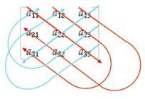pick up the a₃₁, then a₁₃a₃₂a₂₁ by starting at a₁₃ and wrapping around to pick up the a₃₂ and a₂₁. We do the same thing right-to-left for the subtracted terms. This is much easier to visualize than to describe. Determinants of larger matrices are not considered here.

There are just a few rules about manipulating determinants that we need to know:

1. If all the values in a row or column are multiplied by a number, the determinant value is multiplied by that number. Note that here we will always work with a determinant of 0, so we can multiply any row or column by any number without affecting the determinant.
2. The sign of a determinant is changed when two adjacent rows or columns are interchanged.
3. The determinant value is unchanged if every value in any row (or column) is multiplied by a number and added to the corresponding value in another row (or column).

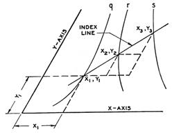That’s it. Now consider the general diagram to the right from Hoelscher showing three curvilinear scales and an isopleth. Similar triangle relations give

(y₃-y₁)/(x₃-x₁)  =  (y₂-y₁)/(x₂-x₁)  =  (y₃-y₂)/(x₃-x₂)

The first two parts of this can be rewritten as a cross product:

(x₃-x₂) / (y₂-y₁)  =  (x₂-x₁) / (y₃-y₂)

and when this is expanded it is equal to the determinant equation

We get this result regardless of which pair we choose to use in the cross product. The x and y elements can be interpreted as the x and y values of f₁(u), f₂(v) and will be f₃( w) if we don’t mix variables between rows (the first row should only involve u, etc.) and if the determinant equation is equivalent to the original equation. This is the standard nomographic form. Here y is not expressed in terms of x as we normally have when we plot points at (x,y) coordinates, but rather x and y are expressed in terms of a third variable, that is, x₁ and y₁ are expressed in terms of a function of the variable u, x₂ and y₂ are expressed in terms of a function of the variable v, and x₃ and y₃ are expressed in terms of a function of the variable w. These are called parametric equations. One way to plot them is to algebraically eliminate the third variable between x and y to find a formula for y in terms of x. Another way is to simply take values of the third variable over some range, calculate x and y for each value, and plot the points (x,y)—a more likely scenario when we have computing devices.

Let’s consider the equation (u + 0.64)^0.58(0.74v) = w that we used earlier to create a parallel scale nomogram. We converted this with logarithms: to 0.58 log (u + 0.64) + log v = log w + log (0.74), or

0.58 log (u + 0.64) + log v – [log w + log (0.74)]  =  0

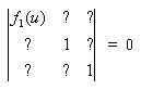
We could have grouped log (0.74) with any term, but we’ll stay consistent with our earlier grouping. This is an equation of the general form f₁(u) + f₂(v) – f₃( w) = 0, so let’s find a determinant that produces this form. We want each row to contain only functions of one variable of u, v or w, so we’ll start with f₁(u) in the upper left corner and 1’s along its diagonal so that the first term of the determinant will be f₁(u).

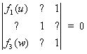
Now let’s set the lower left corner to f₃( w) and the upper right corner to 1 so the last term of the determinant will be –f₃( w):

Now we can place f₂(v) in the middle row somewhere and fill in the rest of the determinant so the terms involving these elements end up simply as f₂(v). Here are a few possibilities that work:

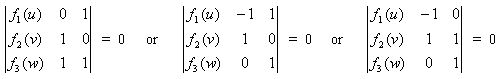
But the second determinant is simply the first one after the third column is subtracted from the second column and the third determinant is simply the second one after the third column is added to the second column. These are operations that will not change our determinant equation as described in our earlier list, so they are all equivalent.

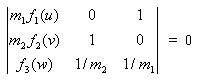
Now we want the flexibility to scale our f₁(u) and f₂(v) by m₁ and m₂ calculated for parallel scale charts as the desired height of the nomogram divided by the ranges of the functions. If we take the first determinant of the three possible ones shown, notice that we can introduce the scaling values without changing the determinant equation if we write it as

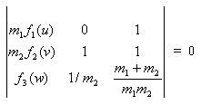
So now we have to convert this to the standard nomographic form having all ones in the last column (and continuing to isolate variables to unique rows). First we add the second row to the third row, where 1/m₁ + 1/m₂ = (m₁+m₂)/m₁m₂:

Then we multiply the bottom row by m₁m₂/(m₁+m₂) and swap the first two columns so that the y column (the middle column) contains the functions:

and we have the determinant in standard nomographic form. The first column represents x values and the second column represents y values of the functions. The scaling factors of m₁ and m₂ result in a scaling factor m₃ for the w-scale of m₁m₂/(m₁+m₂) as we found earlier from our geometric derivation. We had calculated m₁ = 25.72 and m₂=19.93 before, giving m₃=11.23. This determinant also shows that we place the u-scale vertically at x=0 and the y-scale vertically at x=1, with the w-scale at x= m (m₁+m₂) = 0.5634, but in fact we can multiply the first column by 3 to get a scale of 3 inches, and in this case the w-scale lies vertically at x=1.69 inches, and so we end up with exactly the same nomograph we found in Part I using geometric methods.

This was a bit of work, but we have found a universal standard nomographic form for the equation f₁(u) + f₂(v) – f₃( w) = 0 including scaling factors.

Let’s derive a Z chart for division using determinants. For v = w/u, we rearrange the equation so the right-hand term is 0, or uv – w = 0. One possible determinant we can construct is

     

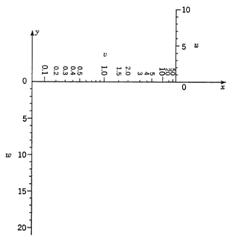
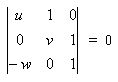
which graphs to the nomogram on the right, a Z chart with a perpendicular middle line. A different determinant would result in a Z chart of the more familiar angled middle line. An interesting aspect of such a chart is that the u-scale and v-scale have different scaling factors despite the fact that they can be interchanged in the equation.

There is a definite knack to all of this, and at this point I’d like to recommend the webpages on nomography by Winchell D. Chung, Jr. at this site. His webpages are quite interesting to read—there are quite a few examples of nomograms, and the determinant approach is used throughout. In particular, he provides other examples of expressing an equation into determinant form here. He also gives a few examples of converting the determinant to the standard nomographic determinant form here, where examples 2 and 3 are from Hoelscher. Most importantly, for equations of several standard formats Chung also reproduces tables that map these equations directly to standard nomographic determinant forms here.

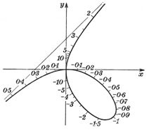
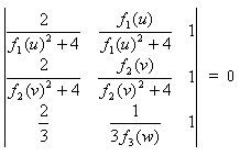
Determinants are most useful when one or more of the u, v and w scales is curved. The quadratic equation w² + uw + v = 0 can be represented as the first equation below, and dividing the last row by w-1 we immediately arrive at the standard nomographic form shown in the second equation:

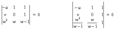
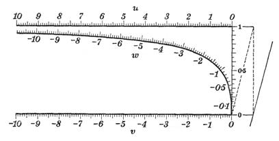The u-scale runs linearly in the negative direction along the line y=1. The v-scale runs linearly in the positive direction with the same scale along the line y=0. The x and y values for the curve for w can be plotted for specific values of w (a parametric equation), or w can be eliminated to express the curve in x and y as

x/y  =  w

y  =  (x/y) / [(x/y) – 1]  =  x / (x – y)

resulting in the figure at the right in which the positive root w₁ of the quadratic equation can be found on the curved scale (the other root is found as u – w₁).

Hoelscher presents the equation for the projectile trajectory Y =  X tan A  –  gX² / (2V₀²cos²A) where A is the initial angle, V₀ is the initial velocity, and g is the acceleration due to gravity. There are four variables X, Y, V₀ and A, so nomographic curves are plotted for different values of A. For an angle of 45º, the equation reduces to

Y  =  X  –  0.0322X2 /V₀²

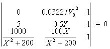
One determinant for this is shown in the first equation below, which can be manipulated into the standard nomographic form shown in the second equation:

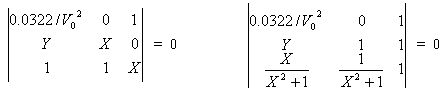
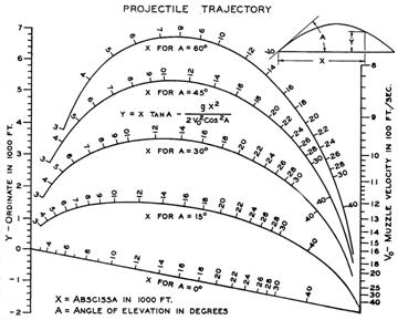Hoelscher assumes -2000<Y<7000 ft and 800<V₀<4000 fps and a chart of 5 inches square, so after some more manipulations (including the swapping of the first two columns) we arrive at the final form:

This is shown as the curve for A=45º along with curves for other angles in this figure (a grid nomogram such as this can be used to handle an equation with more than 3 variables).

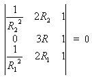
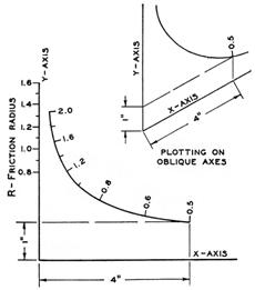
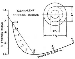
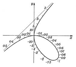
It’s possible to have two or three scale curves depending on how the determinant works out, and it is possible to have two or all three curves overlap exactly. The equation for the equivalent radius of the friction moment arm for a hollow cylindrical thrust bearing is R = 2/3 [R₁³ – R₂³] / [R₁² – R₂²] or 3RR₁²/2 – 3RR₂²/2 – R₁³ + R₂³ = 0, yielding the determinant

Here the R₁ and R₂ scales lie exactly on the same curve. They could have separate tick marks on this curve if they had a different scale, but here they have the same scaling factor. The figures here show the plotted nomogram for perpendicular x and y axes, and also for oblique axes that expand the R-scale to the full height of the nomogram for greater accuracy.

               

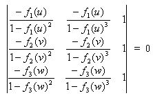
Otto provides an interesting alternate determinant for the equation f₁(u) + f₂(v) + f₃( w) = f₁(u) f₂(v) f₃( w).

The nomogram for the particular equation of this type u + v + w = uvw is shown in this figure, where again two of the three scales overlap. Eliminating f₁(u) from the x and y elements in the first row we find that u lies along the circle given by (x – ¼)² + y² = 1/(4²), and this is correspondingly true for v as well (although in general we have to separately calculate x and y tick marks based on f₁(u) or f₂(v) values).

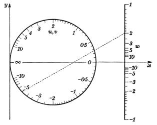
Finally, Otto describes a very interesting determinant that can be created for the equation f₁(u) f₂(v) f₃( w) = 1.

For uvw=1, all three scales coincide and have the same scaling factor, and it turns out that the equation for this curve is x³ + y³ – xy = 0 (called the folium of Descartes). This nomogram is shown as the curled figure to the right.

Determinants provide a creative way of generating nomograms whose designs are varied and interesting.  We can also apply transformations to the x and y elements of the determinants to morph nomograms into shapes that are most accurate for given ranges of the variables or that utilize the available space most efficiently (or are simply more pleasing to the eye).  Transforming nomograms is the subject of Part III of this essay.

<<< Back to Part I of this essay                            >>> Go to Part III of this essay

Printer-friendly PDF of Nomography Parts I-III.