Dead Reckonings

In addition to providing sophisticated nomograms, the use of determinants as described in the previous Part II offers one other huge advantage. Often the scaling factors of variables have to be manipulated to get a nomogram that uses all the available area and yet stretches portions of the curves that are most in need of accuracy; alternatively, there may be a need to bring distant points (even at infinity) into a compact nomogram. This can be done by morphing the nomogram with any transformation that maps points into points and lines into lines. It is also intriguing to consider the aesthetics of such transformations, creating eye-catching nomograms as an artistic process.

This final part of the essay reviews the types of transformations that can be performed on a nomogram, and it concludes by considering the roles of nomograms in the modern world and providing references for further information.

There are several standard transformations of the Cartesian coordinate system that preserve the functionality of nomograms. After they are presented we will walk through a sequence of these to see their effects on the shape and scales of a nomogram.

Translation

We can translate the nomogram laterally, which is equivalent to translating the x-y axes to new x’-y’ axes. We can add c to all determinant elements in the x column and d to all determinant elements in the y column to shift the axes left by c and down by d (or in other words shift the nomogram right by c and up by d).

x_n‘ =  x_n + c

y_n‘ =  y_n + d

Rotation

We can rotate the nomogram about the origin of the axes by an angle θ (positive for counter-clockwise rotation) by replacing each determinant element x_n in the x column and the each determinant element y_n in the y column with

x_n‘ =  x_n sin θ  +  y_n cos θ

y_n‘ =  x_n cos θ  –  y_n sin θ

Stretch

We can stretch a nomogram in the x direction by multiplying each determinant element in the x column by a constant, and likewise for the y direction.

x_n‘ =  cx_n

y_n‘ =  dy_n

Shear

Shear is a slewing of perpendicular axes to oblique axes or vice-versa. This is perhaps best understood by referring to this figure showing a shear from one set of axes x-y to another set x’-y’ in which the x’ axis is canted at an angle θ to the x axis but the y’ axis aligns with the y axis. For this case,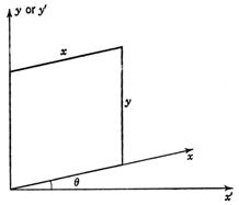

x_n‘ =  x_n cos θ

y_n‘ =  y_n + x_n sin θ

Shear can be used to convert a traditional Z chart with a slanting middle line to one with a perpendicular middle line and vice-versa. It could have been used to convert the determinant for the earlier nomogram of equivalent friction radius to plot it relative to the oblique x’-y’ axes rather than to the perpendicular x-y axes.

Projection

Referring to the first figure below, a projection uses a point P (called the center of perspectivity) to project rays through points of a nomogram in the x-y plane to map them onto the z-y plane (also called the x’-y’ plane), foreshortening or magnifying lines in varying amounts in the x’ and y’ directions. It is also possible for P to lie above the x-y plane, where rays from points on the nomogram pass through P to the x’-y’ plane as shown in the second figure. (This can be used to convert a nomogram in the shape of a trapezoid to a rectangular one, changing scale resolutions to maximize the available space, but we will see an easier method later.) In either case, for a P location (x_P,y_P,z_P) and a nomogram x-element x_n and y-element y_n,

x_n‘ =  z_P x_n / (x_n – x_P)

y_n‘ =  (y_P x_n – x_P y_n) /  (x_n – x_P)

    

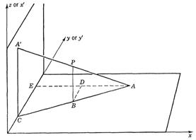
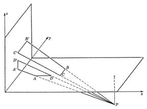
The line BD under P in the second figure never maps onto the x’-y’ plane because it is parallel to that plane—it is a “straight line at infinity” and will become important in our example below.

A Transformation Example

Epstein outlines a sequence of transformations to convert a nomogram for the equation q² – aq + b = 0 to a more convenient circular form. Unfortunately, he provides only the final nomogram, so I have taken up his challenge and traced through the details of each step while creating my own intermediate nomograms. These nomograms were created using the freely-available LaTeX typesetting engine and the free vector drawing package TiKz, which supports plotting parametric functions and has enough flexibility to draw and nicely label tick marks on the curves. Excel and MATLAB, for example, can plot parametric functions but do not appear to support labeled tick marks on the curves corresponding to the parametric variable. Chung uses Python code to create his nomograms (described here) and there is a very powerful Python program to plot nomograms here. An online tool to create custom, interactive parallel scale nomograms only can be found here. I find that the LaTeX code is quite simple and very flexible and is especially convenient for those of us who already use LaTeX to create technical articles. My LaTeX code that created the nomograms below can be found here.

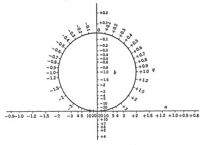
A determinant representing the equation q² – aq + b = 0 can be constructed (and verified it by multiplying it out) as

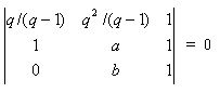
(Note: In all determinants in this essay the x elements are in the first column and the y elements in the second column, which follows most presentations but is reversed from Epstein’s.)

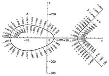
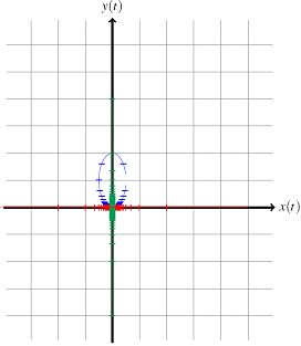
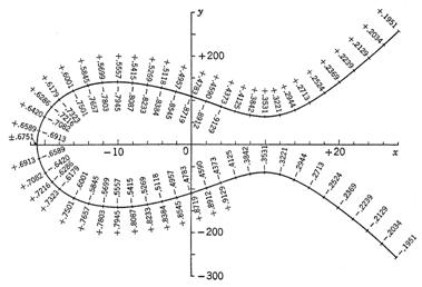
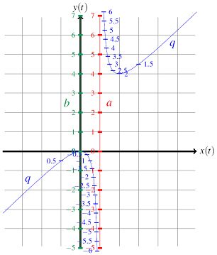This nomogram is plotted in the figure to the right (the x-y axes and grid would be deleted from the final nomogram). The q-scale is found in practice by taking a range of q values and calculating x = q / (q+1) and y = q² / (q-1) as a coordinates to plot, but if we eliminate q between the two parametric equations we arrive at x² – xy + y = 0, demonstrating that the q-scale is in fact a hyperbola. A straightedge placed across any two values of a and b will intersect the q-scale in two points if there are two real solutions, one point if there is a double real root, and no points if there are no real roots. However, the layout of the q-scale is problematic, as the two halves stretch toward infinity very quickly and it is not possible to accurately locate q points for isopleths near the asymptotes of the hyperbola. So we will transform this nomogram into one in which the q-scale is finite. The labels for the tick marks will not be displayed on the following plots, but the tick mark spacing and colors will provide a guide for how the curves are re-mapped.

First we will rotate this nomogram clockwise by 45° (or θ = -45°) and stretch it in both dimensions by 2^1/2 for a reason that will become apparent in the next transformation. Since cos -45° = 2^-1/2 and sin 45° = -2^-1/2, the earlier rotation formulas after the stretch become

x_n‘ =  x_n  +  y_n

y_n‘ =  –x_n +  y_n

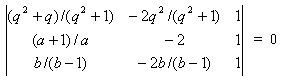
Performing this substitution for the x element and y element of each row of the determinant, we arrive at

which is plotted on the right.

We rotated the nomogram because we wanted a vertical line (say, x=1) that does not intersect the hyperbola. A projection transformation can convert a scale with two branches like this hyperbola into a single connected scale (an ellipse) if a straight line separating the two branches is projected to infinity, that is, if the line is parallel to the y-z axis (which x=1 is) and the projection point 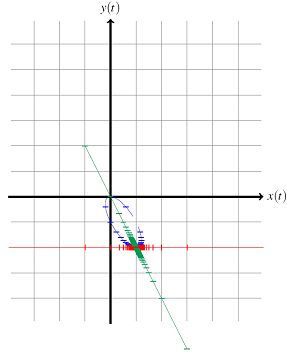P is located directly above or below it in its z value (as the line BD in the earlier projection figure). Choosing P = (1,-1,1), the earlier projection formulas become

x_n‘ =  x_n / (x_n – 1)

y_n‘ =  (-x_n – y_n) /  (x_n – 1)

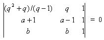
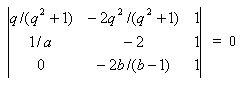
and the determinant becomes

and the ellipse magically appears in the plot on the right.

Now let’s shear the nomogram so the green b-scale lies on the y-axis while keeping the red a-scale parallel to the x-axis. The shear formulas are slightly different as we are shearing to the y-axis, 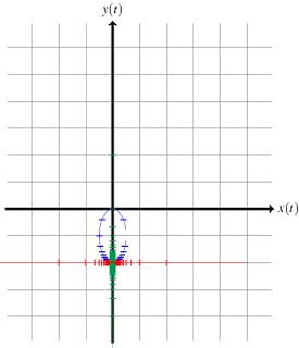and for a b-scale slope of –½ they reduce to:

x_n‘ =  x_n  + y_n / 2

y_n‘ =  y_n

and the determinant becomes

which is plotted on the right.

Now we’ll translate the nomogram upward by 2 to place the intersection point on the origin.

x_n‘ =  x_n

y_n‘ =  y_n + 2

This is plotted on the right.

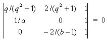
And finally we shrink the nomogram in the y 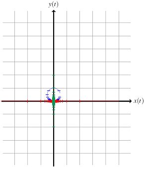direction by a factor of 2 to get a circular scale for q.

x_n‘ =  x_n

y_n‘ =  y_n / 2

yielding

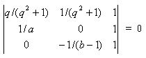
The figure on the right is the plot of my final determinant, and by changing the scales of the axes we arrive at Epstein’s figure below.

The entire range of q from -∞ to +∞ is now represented in a finite area, and certainly the range less than 1.5, which veered to infinity in our original nomogram, is nicely accessible. 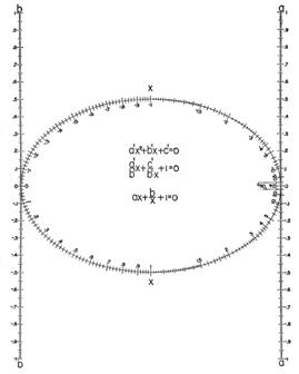The larger numbers are not as accessible, but the ranges can be skewed to spread out any range by multiplying the original equation by a constant. We could have stopped at any of the nomograms containing an ellipse, but it is easier to draft the circle. An elliptical nomogram for the quadratic equation ax² + bx + c = 0 is shown here for comparison.

It’s interesting to play around with a straightedge on the circular nomogram we derived above to see that it works. In particular, an isopleth through an a-value and b-value will just touch the q-circle if the discriminant from the quadratic formula is 0 (for the equation Ax² +Bx + C = 0, the discriminant is the value B²-4AC whose square root is taken in the quadratic formula, or a²-4b here). When the discriminant is less than zero the isopleth misses the q-circle, denoting no real roots, and when it is greater than zero it crosses two real roots on the q-circle.

And in fact if you eliminate the a-scale, then the b-scale represents the product of two numbers on the q-circle. This is because if we have two solutions q₁ and q₂ of q² – aq + b = 0, then the equation can be written as (q – q₁)( q – q₂) = 0. Multiplying this out and equating terms to the original equation, we find that b = q₁q₂ and a = q₁+q₂. The geometric layout of this nomogram is really the traditional meaning of a circular nomogram (two scales on the circle, one on a nearby line), and it turns out that any three-line parallel scale nomogram can be transformed into a circular nomogram. Generally the two scales on the circle do not have the same values, so tick marks on both sides of the circumference are needed.

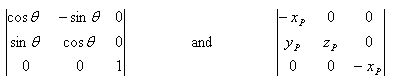
The transformations we have discussed can also be represented as matrices. Transformations are performed by matrix multiplication of the transformation matrix and the nomogram determinant. Two or more transformations can be combined by multiplying their transformation matrices. It often happens after such a matrix multiplication that the nomogram determinant needs to be manipulated again into the standard nomographic form. For example, the transformation matrices for rotation and projection are

It is possible to use matrix multiplication to map a trapezoidal shape (such as the boundaries of a nomogram that does not occupy a full rectangle) into a rectangular shape. This would increase the accuracy of the scales that can be expanded to fill the sheet of paper. Consider the following matrix multiplication:

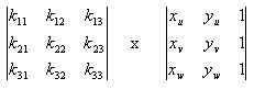
By the rules of matrix multiplication and some manipulation of the result, each y’ and x’ in the resulting matrix can be represented as

x’ =  (xk₁₁ + yk₂₁ + k₃₁) / (xk₁₃ + yk₂₃ + k₃₃)

y’ =  (xk₁₂ + yk₂₂ + k₃₂) / (xk₁₃ + yk₂₃ + k₃₃)

Now if we want to remap an area such that the points (x₁,y₁), (x₂,y₂), (x₃,y₃) and (x₄,y₄) map to, say, the rectangle (0,0), (0,a), (b,0) and (b,a), we insert the final and initial x’s and y’s into the formulas above, giving us eight equations in nine unknown k’s. So we choose one k, solve for the other eight k’s and multiply the original nomogram determinant by the k matrix and convert it back to standard nomographic form, then replot the nomogram—a fun way to spend an afternoon.

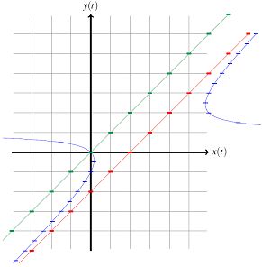
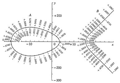
There are non-projective transformations as well that can be used to create nomograms in which all three scales are overlaid onto one curve (although the third will have different tick marks). This is highly mathematical and involves things called Weierstrass’ Elliptic Functions, so Epstein is a resource if there is interest in the details. Epstein provides nomograms of this sort for the equation u + v + w = 0 (which can be generalized to any equation of this form, including ones in logarithms). In the first figure below, the isopleth must cross two numbers on one scale and a third number on the other overlaid scale (such as u = +0.2524, v = +0.3842 and w= -0.6366). In the second figure the isopleth crosses two curves containing three scales. Ignore the numbers on the x-axis and y-axis—these relate to the function used to derive the nomograms. I’m showing these simply to demonstrate the advanced mathematics that was targeted at nomographic construction at one time. (Please see my later essay A Zoomorphic Nomogram for a detailed discussion on using these elliptic functions to create a nomogram.)

Transformations provide a creative way of morphing nomograms into designs that are most useful, such as increasing the accuracies of particular ranges of variables. They also allow us to create nomograms that are eye-catching and artistic.

The Status of Nomograms

Today the use of nomograms seems scattered at best. Chung’s interest in nomograms shown here grew from his desire to provide quick and easy calculations of hit strength, etc., in strategic wargaming. There are many simple nomograms that exist for doctors to quickly assess attributes and probabilities, such as here (or here if you can’t draw a line), here, here, and here. A Body Mass Index (BMI) nomogram is common (such as here) and is derived in this PowerPoint presentation on nomograms. There are also some engineering nomograms found here and there online (such as here, here, here, here, here, and there).

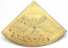
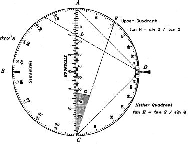I first heard of nomograms in the context of sundials. As Vinck and Sawyer describe (see references), Samuel Foster published a treatise in 1638 titled “The Art of Dialling” that contained a dialing scale for the construction of horizontal, vertical and inclining sundials as shown in the figure from Vinck to the right. Foster’s construction scale is actually a circular nomogram, a tool discovered nearly 300 years earlier than its attributed discovery by J. Clark in 1905! Sawyer writes that Foster did write of the more general computing applications of his scale. Here an isopleth from one point on a perimeter scale through a point on the middle scale will cross their product on the other perimeter scale, and with suitable trigonometric scaling one can lay out hour lines on a wide variety of sundials. Certainly many sundial designs (nearly all) rely on graphical plots with the gnomon shadow or a weighted, hanging string serving as the isopleth. Card dials are particularly complicated because they map a 3-D geometry to a 2-D plane, as you can see on this webpage. Sawyer has designed a few dials that employ nomograms, two of which are shown below.

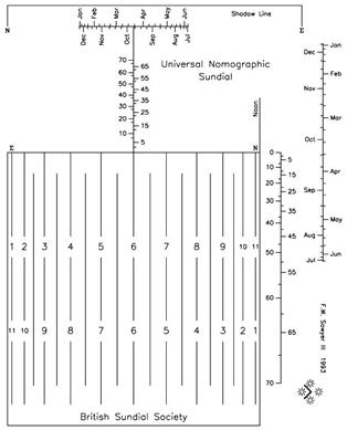
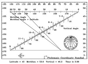
Masse uses the same projection transformation method as we did to create a sundial in which the gnomon tip shadow during the day traces a circle rather than a hyperbola on the face of the dial. My interest in nomography (including the transformation techniques) and my efforts to plot nomograms using the LaTeX typesetting engine are partly due to my intention to create new sundial designs based on nomograms.

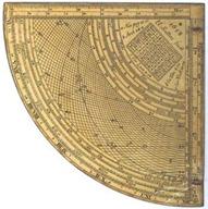
The use of analog graphic calculators is actually much older—the quite complicated grids and curves on old astrolabes and quadrants, as shown below, effectively serve as nomograms. There are also curves on the backs of most astrolabes to convert equal hours to unequal hours using the alidade (the sight on the back) as an isopleth, and the qibla diagram on the back of Islamic astrolabes provides the direction to Mecca for any hour of any day by using the alidade when the astrolabe is aligned correctly.

                 

And I think there could be more applications today. I was at a picture framing store while I was writing this essay to get a matte board cut as a frame for some calligraphy created by my son. The pricing was based on three variables (the window height, the window length and the border width) and possibly the matte board type. Everyone who came up to get a price for a certain configuration or a variety of configurations had to wait while the clerk wrote down the three parameters, punched them into some formula on a calculator, and referred to a chart to find the corresponding price in quarter-dollars. I was thinking the whole time that having photocopies of a nomogram laying around would let customers use a straightedge (and there are a lot of those in a framing store!) to figure the pricing out and quickly optimize their parameters without having to wait in line, and it would certainly be faster for the clerk.

But nomograms have their own intrinsic charm. As a calculating aid a nomogram can solve very complicated formulas with amazing ease. And as a curiosity a nomogram provides a satisfying, hands-on application of interesting mathematics in an engaging, creative activity.

References

Update 10/17/2008: Leif Roschier, author of the powerful Pynomo software for creating nomograms, has updated his site found here with beautiful nomograms he has created. Be sure to visit the Basics and Examples links on his site. If you click on the Software Documentation link you can select nomograms by type to view as well. Leif also maintains a forum on nomography found here.

Douglass, Raymond D. and Adams, Douglas P. Elements of Nomography. New York: McGraw-Hill (1947). This book is as concerned about the drafting aspects of nomograms as with their (exclusively geometric) derivations. The printed forms it champions for calculating nomograms are more trouble than they are worth, in my opinion.

Epstein, L. Ivan. Nomography. New York: Interscience Publishers (1958). An advanced book that treats determinants throughout as well as projective transformations. It should not be the first book or two to read on nomography.

Hoelscher, Randolph P. et al. Graphic Aids in Engineering Computation. New York: McGraw-Hill (1952). The best all-around book on nomography of the ones listed here. Geometric derivations are given first and determinants introduced later in a very understandable presentation. It also contains a very interesting chapter on special slide rules created for solving particular engineering equations.

Johnson, Lee H. Nomography and Empirical Equations. New York: John Wiley and Sons (1952). A good, solid reference that is very readable. Uses geometric derivations throughout (no determinants) and treats all the common nomographic forms.

Levens, A.S. Nomography. New York: John Wiley and Sons (1937). A very readable book that is organized in a very convenient manner based on equation types. A very nice collection of nomogram examples of various types is presented in the Appendix. For nomograms created from geometric derivations only (and only the most sophisticated nomograms types really require solutions by determinants) this is an excellent reference book with many examples.

Masse, Yvon. Central Projection Analemmatic Sundials, The Compendium, Journal of the North American Sundial Society, Vol. 5, No. 1, Mar. 1998, pp.4-9.

Otto, Edward. Nomography (International Series of Monographs in Pure and Applied Mathematics).New York: Macmillan (1963). An advanced but (with some work) a readable book that uses determinants throughout to create nomograms as well as projective transformations to square them up or expand scales for greater accuracy. There is a long, interesting chapter on problems of theoretical nomography, such as determining what equation forms can be expressed as nomograms.

Sawyer, Fred. Ptolemaic Coordinate Sundials, The Compendium, Journal of the North American Sundial Society, Vol. 5, No. 3, Sep. 1998, pp.17-24. Describes three sundials incorporating nomograms.

Sawyer, Fred. A Universal Nomographic Sundial, Bulletin of the British Sundial Society, Oct. 1994. 94(3):14-17, also in Sciatheric Notes, a collection of sundial articles by Fred Sawyer from this publication. This collection and all the sundial-related articles referenced here can be found in the outstanding North American Sundial Society Repository CD orderable on the NASS site.

Vinck, Rene J. Samuell Foster’s Circle, The Compendium, Journal of the North American Sundial Society, Vol. 8, No. 3, Sep. 2001, pp.7-10. Also see Fred Sawyer’s The Further Evolution of Samuel Foster’s Dialing Scales that follows this article in the same issue of the journal.

Blog Update (not yet in the current PDF file):  Google has digitized the entire book Graphical and Mechanical Computation (1918) by Joseph Lipka that can be read or downloaded here (link updated 1/27/08). Chapters 3-5 on nomography have example after example of creating nomograms from the geometrical formulas.

 <<< Back to Part II of this essay            >>> A Zoomorphic Nomogram essay

Printer-friendly PDF of Nomography Parts I-III.