Dead Reckonings

In Part III of my essay on The Art of Nomography, I mentioned the use of Weierstrass’ Elliptic Functions to create a nomogram composed of three variable scales overlaid onto a single curve. In particular, Epstein describes using this family of functions to create a nomogram for the equation u + v + w = 0, adding that the formula can be generalized for functions of these variables. This topic generated some interest, and it certainly is interesting to me, so I’ve explored it in more detail by designing a single-curve nomogram based on functions of u, v and w. This essay describes the procedure I followed to create a “fish” nomogram (found here) manifesting the formula for the oxygen consumption of rainbow trout as a function of weight and water temperature—a modest attempt to blend art with artifice.

To review, Epstein displays two examples of nomograms based on these elliptic functions as shown below. A line (isopleth) crossing any three points anywhere on the entire curve produces three label values that add to zero. When two of the values are identical, the isopleth is drawn tangent to the curve at that point. In the first figure, the isopleth must cross two numbers on one scale and a third number on the other overlaid scale (such as u = +0.2524, v = +0.3842 and w= -0.6366). In the second figure the isopleth generally crosses both curves, although it could just cross the rightmost curve three times along the shallow curve if the scale were stretched enough to distinguish the crossing points.

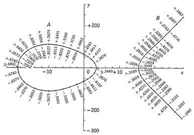
The values on the x and y axes are not used in reading the nomogram but rather relate to the plot of the Weierstrass’ Elliptic Function providing the outline of the nomogram:

The first plot above is for g₂ = 1200 and g₃ = -12000 (with one real root around x = -21), while the second is for g₂ = 1200 and g₃ = -4000 (with three real roots at about x = -19, 3.5 and 15.5). Somewhere between these two functions (at g₂ = 1200 and g₃ = 8000) the two curves just touch, representing a double real root. These plots were presented as a demonstration of the level of some of the mathematics under development for nomograms at the time.

Looking at this in more detail now, the scale values for all points on these curves are calculated from

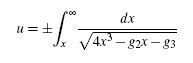
Like most things elliptic in mathematics, this integral cannot be solved directly but must be numerically computed to the accuracy desired. Epstein’s book from 1958 discusses methods of approximating the integral in different ranges; today we have computer programs that can easily perform numerical integration. In practice the positive-value scale above the x-axis in the first figure above is initially calculated from this integral. Now the difference in any two lower scale values is the negative of that for the upper scale, so the positive-value scale that wraps below the x-axis is calculated at each x by adding the difference between the value at y=0 and the value at x on the upper scale to the value at y=0. For example, the value +.7803 on the lower scale is found by adding  (0.6751 – 0.5699) to 0.6751, and in this way the entire positive-value scale can be labeled. The negative-value scale halves are simply labeled with negative values of their opposite positive-scale halves.

Epstein provides a proof that these scales on this family of curves produce a nomogram in which three crossed values add to zero.

Now assume we have the more general formula f(r) + g(s) + h(t) = 0. We can then assign scale values for r, s and t such that f(r), g(s) and h(t) result in the original scale values found above, and we can use the same curve. Notice in the first figure above that when an isopleth intersects the upper curve at two or three points, the negative-value is added to the two positive-values. So we can map, say,  f(r) to the negative-values and g(s) and h(t) to the positive-values. However, when an isopleth intersects the lower curve in two or three points, two negative-values are added to a positive-value, so we can continue to map, say, f(r) and g(s) to the same negative- and positive-values as they wrap continuously around through the lower curve, but h(s) has to change its mapping to negative-values. This took me a while to realize, and it means that h(s) scale values will be discontinuous when crossing the x-axis. We will see how I handled that.

Let me say a word about the software tools we will use in creating the fish nomogram. I hasten to add that nomograms can be calculated and plotted by hand or in Excel or PowerPoint or Word or AutoCAD or Visio or whatever—I use tools that I’m familiar with from other applications and these will probably be different tools than you would use. The only real software need for this project is a math program to do numerical integration to find the default scale values for a given set of g₂ and g₃, which only needs to be done once. However, one of my aims was to create a general set of tools that allow me to quickly create new nomograms based on elliptic functions.

So here are my specific tools. All software listings will be linked in this essay. The MATLAB program is used to perform the numerical integration and to provide plots for solving a system of equations for the desired scale ranges. This is an expensive program, but GNU Octave is a free, open-source program for various platforms that is mostly compatible with MATLAB scripts. The mathematics typesetting engine LaTeX is used to output the PDF of the actual nomogram. I use the free MiKTeX distribution of LaTeX, and the free, matching editor and user interface TeXnicCenter. I also use the powerful TikZ drawing package for LaTeX, which also provides plotting capability for PDF output once the free gnuplot program is installed. LaTeX has limited programming capability, so I use a separate program to calculate label values and coordinates for the scales and store them into text files that are read in by the LaTeX program. This program is written in the free, open-source scripting language Tcl, for which I use the free ActiveTcl download. However, Tcl and its companion TK are installed by default on most Unix systems and on Mac OS X.

To begin, we need to find values of g₂ and g₃ for the elliptic function that provide the best overall fish outline—I settled on g₂=1200 and g₃=-8500. (I used the plot command in LaTeX that you will see in the later listing, but any plotting program will do.) We can calculate the positive-values on the upper curve for each x-value by running the script below in MATLAB.

---

g2 = 1200.0;
g3 = -8500.0;
h=@(x) (1.0 ./ sqrt(4*x.^3-g2*x-g3));
for xvalue = -40:1:40
% Output x
xvalue
% Do numerical integration and output result
result = quad(h,xvalue,10000000000)
end

---

And, yes, I did have to take the integration all the way out to x=10,000,000,000 to get the answer to four decimal places. But this was completed instantly in MATLAB on my PC, indicating that the program does an intelligent distribution of integration intervals. This script prints out the values to the screen, but I also added some script lines to print the output values to a file as well for convenience—this longer version can be found here (unzip it to run it in MATLAB). The presence of a non-zero imaginary component in any result indicates that x lies off the end of the curve and there is no y-value to plot.

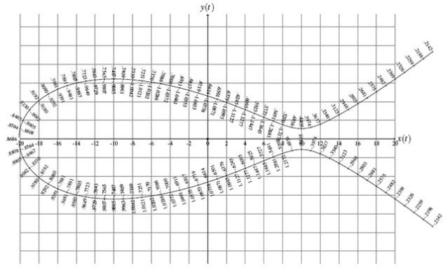
The wrap-around part of the positive-value scale as well as the negative-value scale and its wrap-around to the upper curve are found by simple manipulations of these numbers as described earlier. Below is the nomogram for u + v + w = 0 for g₂=1200 and g₃=-8500. Click here for a full-resolution version.

Looks like a fish to me. But we want to develop this nomogram for a more general equation than u + v + w = 0. I found a fish-related equation developed by Liao that provides the oxygen consumption rate O₂ in weight units of dissolved oxygen (DO) per 100 weight units of fish per day as a function of water temperature T in °F and average individual fish weight W in lbs.:

O₂ = K Tⁿ  W^m

where the rate constant K and the slopes m and n for rainbow trout are given by:

for T>50:  K = 3.05×10^-4,  n = 1.855,  m = -0.138
for T<50:  K = 1.90×10^-6,  n = 3.130,  m = -0.138

Apparently this is important in the design and calibration of aerators for rainbow trout “racetracks” at trout farms.

Since there is a different equation for T<50 than for T>50, we can take advantage of that to skirt the difficulty of the discontinuity of one of the positive-value scales as it wraps around from the upper curve to the bottom curve as mentioned earlier. We will implement the equation for T>50 on the upper curve, with T using a positive-scale, W using a negative-scale, and O₂ using a positive-scale and wrapping around the lower curve continuing as a positive-scale. So for T>50 the isopleth has to cross two or three points above the x-axis since there are no W or T scales on the lower curve. This allows the third scale O₂ to wrap around and maintain positive values. The equation for T<50 will be implemented on the lower curve, with T′ and W′ using negative-value scales and O′₂ using a positive-value scale and wrapping around to the upper curve continuing with the positive-value scale.

Using logarithms the oxygen consumption equation can be cast in the correct format for the nomogram:

n log T  +  m log W  +  (log K – log O₂)  =  0

The term log K could be paired with any term, actually.

So we need to place labels T, W and O₂ on the plot above such that each corresponding term in this equation is equal to the u, v and w values shown in the plot for u + v + w = 0. Setting each term in the equation above to a corresponding variable u, v or w, we have

u  =  n log T                      or      label  “T” =  e ^u/n
w  = m log W                   or      label  “W” =  e ^w/m
v  =  log K – log O₂         or      label  “O₂” =  e ^{log K  –  v}  =  K e ^–v

Consider the upper curve only for the moment. Let’s assign T to the positive-value scale, W to the negative-value scale, and O2 to the positive-value scale that wraps around to the lower curve. The range of the u scale is 0.2142 to 0.8686 for the upper curve. The range for the w scale is -0.8686 to -1.5230 (at x=24), and the range of the v scale is 0.2142 to 1.5230 if we let this scale wrap all the way around to x = 24. With these limits, the above equations for T>50 produce ranges of 4.7217<W<62083.3 and 1.1224<T<2.2839, wildly different from what we want for the nomogram.

But there are at least two ways to change the range of our T and W scales without changing the basic equation u + v + w = 0. First, we can multiply u, v and w by the same constant A. Second, we can add offsets u₀ and w₀ to u and w if we subtract (u₀ + w₀) from v.

According to Wikipedia, the world record rainbow trout was a 43.6 pounder caught from the shore at Lake Diefenbaker, Saskatchewan in June, 2007. If we desire ranges of  50<T<100 and  0.5<W<50, say, then we want from the above equations

e ^{A(0.2142 + u₀) / 1.855}  =  50
e ^{A(0.8686 + u₀) / 1.855}  =  100
e ^{A(-.0.8686+ w₀) /  (-0.138)} =  0.5
e ^{A(-1.5230 + w₀) / (-0.138)}  =  50

This is an over-determined system comprising 4 equations with only 3 variables to define: A, u₀ and w₀. There’s no guarantee that even 4 variables would allow this system of equations to be solved, so unless one of the equations happens to be a duplicate of another there’s no way we will be able to exactly solve this system. The best we can do is to find values of A, u₀ and w₀ that will approximately provide the ranges we want. The way to do this is to move all the terms to left sides of the first two equations and plot them against each other (setting y=A and x=u₀) to see where they intersect, thereby solving for A and u₀ for these first two equations. Then we do the same for the second pair of equations, solving for A and w₀ for these equations. Then we cross our fingers and hope that the values of A are about the same so we can pick one that roughly satisfies all 4 equations.

A MATLAB script to plot the two sets of equations on a single grid is shown below, followed by the resulting plot (after some interactive editing to add grids, colors and a legend).

---

hold on; % To overlay multiple plots
syms x y;
eq1 = ‘exp(y*(.2142+x)/1.855)-50’;
eq2 = ‘exp(y*(.8686+x)/1.855)-100’;
ezplot(eq1,[-10,10,-6,6]), ezplot(eq2,[-10,10,-6,6]);
syms x y;
eq1 = ‘exp(y*(-.8686+x)/-.138)-0.5’;
eq2 = ‘exp(y*(-1.523+x)/-.138)-50’;
ezplot(eq1,[-10,10,-6,6]), ezplot(eq2,[-10,10,-6,6]);

---

Looking at the intersections of the two pairs of plots, the values of A (the y-value) for them are remarkably close. So we pick the intersection most sensitive to differences (that for the second pair of equations) and we find approximately that A = 0.9725 and w₀ = 0.9725 by interactively zooming into the plot. (The fact that these two values are identical is coincidental—I did these plots for several different ranges and they were always different). For this value of A the average value of u₀  (the x-value) for the first two equations is about 7.65.

The only rigid constraint on our range is the minimum value of 50 for T, so we need to adjust u₀ to achieve this. Substituting A = 0.9725 into the first of the 4 equations above we find that u₀ = 7.2478 provides a value of 50 on the right side. This means that v₀ = -(7.2478 + 0.9725) = -8.2203, and we end up with the following scale equations for the upper curve:

T = e ^{0.9725 (u + 7.2478) / 1.855}               using positive-scale values of u
W = e ^{0.9725 (w + 0.9725) / (-0.138)}        using negative-scale values of w
O₂ = 3.05×10^-4 e ^{0.9725 (v – 8.2203)}    using positive-scale values of v

which gives ranges of 50<T<70.46 and 0.4809<W<48.40, which is acceptable. And we can now list these values in place of the original u, v and w values on our upper fish outline and we have a nomogram for the T>50 equation!

We repeat all this for the lower curve for the equation for T<50. We assign T′ to the negative-value scale on this lower curve, W′ to the negative-value scale as well, and O′₂ to the positive-value scale that wraps around to the upper curve. With ranges of  32<T′<50 and  0.5<W′<50, say,

e ^{A(-0.8686 + u₀) / 3.130}  =  32
e ^{A(-0.2142 + u₀) / 3.130}  =  50
e ^{A(-.0.8686+ w₀) / (-0.138)} =  0.5
e ^{A(-0.2142 + w₀) / (-0.138)}  =  50

We choose A = 0.9725 as before (although we have the freedom to choose a different A for the lower curve), with w₀ = 0.335 and u₀ ≈ 12.3 from the MATLAB plots. To have a maximum T of 50, u₀ = 12.805, so v₀ = -13.14 and we arrive at the following scale equations for the lower curve (with primes on the variables to distinguish this set of scales):

T′ = e ^{0.9725(u + 12.805) / 3.130}            using negative-scale values of u
W′ = e ^{0.9725(w + 0.335) / (-0.138)}        using negative-scale values of w
O′₂ = 1.90×10^-6 e ^{0.9725 (v – 13.14)}    using positive-scale values of v

which gives ranges of 40.8<T′<50 and  0.4269<W′<42.96, which we’ll accept as well. And now we can list these values in place of the original u, v and w values on the lower fish outline for the T′<50 equation.

A Tcl script is used to perform the calculations of T, W and O₂ and store the values along with their scaled x and y coordinates and angles. The script reads in a set of prepared files that must be placed in the directory of the Tcl script. These files contain the unscaled values of u, v and w for u + v + w = 0 when g₂=1200 and g₃=-8500 as calculated by MATLAB and shown in the black-and-white plot above (click on the filenames to see their contents):

• positive_values_uppercurve_g2_1200_g3_-8500  —  (x,labelvalue) pairs
• negative_values_uppercurve_g2_1200_g3_-8500 —  (x,labelvalue) pairs
• positive_values_lowercurve_g2_1200_g3_-8500 —  (x,labelvalue) pairs
• negative_values_lowercurve_g2_1200_g3_-8500 —  (x,labelvalue) pairs

The following files are output to this same directory by the Tcl script for reading by the LaTeX files when placing the tickmarks and labels on  the elliptic function plot. Separate files for each portion of the curve are created to ease LaTeX code.

• uppertickmarks —  (x,labelvalue) pairs
• T_upper —  (xcoord,ycoord,labelvalue,angle)
• W_upper —  (xcoord,ycoord,labelvalue,angle)
• OX_upper_upper —  (xcoord,ycoord,labelvalue,angle)
• OX_upper_lower —  (xcoord,ycoord,labelvalue,angle)
• T_lower —  (xcoord,ycoord,labelvalue,angle)
• W_lower —  (xcoord,ycoord,labelvalue,angle)
• OX_lower_lower —  (xcoord,ycoord,labelvalue,angle)
• OX_lower_upper —  (xcoord,ycoord,labelvalue,angle)

The Tcl script can be found here (unzip to run it). It performs the required calculations, formats the labels as 4-digit strings with a decimal point, scales the x and y coordinates for the final plot, and calculates the angles for tickmarks and labels from the slopes between neighboring points.

These output files are then copied to the directory of the LaTeX script, which plots the curve and reads label values and coordinates from the files, placing the tickmarks and labels at the required positions and angles on the curve. The script also creates the fish features such as the eye and fins, and it routes labels around the fins and adds lines within the fins to relate these labels with their tickmarks. Finally, it adds the title, legend and scale names. This LaTeX script can be found here (unzip to run it).

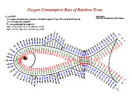
The final nomogram in full resolution can be downloaded from here. A reduced, lower quality version is shown below for discussion purposes. The scale colors are meant to suggest a rainbow trout, but I wanted long scales on the tail so I replaced the rounded tail of the trout with a V-shaped tail. So you should consider this a simple fish illustration.

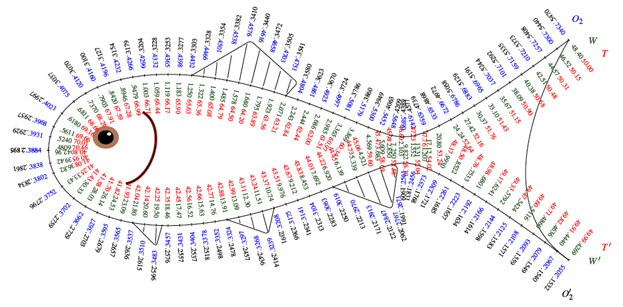
Here the scales on the nomogram marked O₂, T and W apply to T>=50 (as you can see since the T scale starts at 50.00 and goes up), where the blue O₂ scale also wraps around the bottom of the fish. The scales O’₂, T’ and W’ apply to T<50. (I manually changed the T label on the lower curve from 50.00 to 49.99 to avoid confusion on which T scale to use.) All the scales reside along the main fish body, and the lines through the fins are just pointers from the outer scales to their tickmarks. An isopleth crossing any three points on the primed set of scales or three points on the unprimed set of scales will provide three values that solve the oxygen consumption equation.

One of the intriguing features of nomograms is that they can solve for any variable in the equation even when there is no explicit solution for that variable. In this nomogram, any isopleth that does not cross the center line will encompass 6 possible combinations of T, W and O₂ locations (O₂TW, O₂WT, WO₂T, TO₂W, TWO₂, WTO₂). An isopleth crossing the center line will have only 2 possible combinations since O₂ or O’₂ must lie by itself at one end of the isopleths (TWO₂, WTO₂). All combinations in our ranges are available this way except for isopleths near the mouth at an angle where the isopleth misses the end of the tail. The ranges could have been mapped to stop at the top of the head rather than the mouth if this were really an issue. Compare this with the situation in the first figure from Epstein, in which there are many possible isopleths that intersect the curve in only two points.

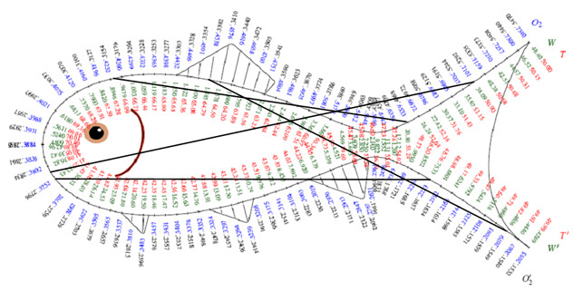
Some possible isopleths are shown in the figure above. A significant amount of testing demonstrates that the nomogram works great, which is still a bit surpris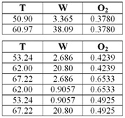ing to me. As an example, consider the isopleth in this figure whose right end touches the upper edge of the tail closest to the tip. This line provides oxygen consumption values for the two variable combinations listed in the upper table on the right.

As another example, the isopleth that crosses three points on the upper curve provides the six variable combinations shown in the lower table on the right.

One thing that was impressed upon me during this exercise is the amount of work needed to create a nomogram that is effective and simple to use, regardless of the shape! In retrospect I wish I had expended my efforts on an equation more useful or more interesting to me. I could have rotated the plot 90° clockwise, drawn rocket fins rather than fish fins, and nomographed an equation related to rocketry, astronomy or space science. But my objective was to learn how to create nomograms based on Weierstrass’ Elliptic Functions, which has happened, and software components now exist to quickly create other nomograms of this sort. It’s also true that I have never before seen a nomogram in the shape of anything specific, although it seems to me that even traditional nomograms could be incorporated in some way into drawings of objects they represent.

References

Epstein, L. Ivan. Nomography. New York: Interscience Publishers (1958). An advanced book that treats determinants throughout as well as projective transformations. It should not be the first book or two to read on nomography.

Soderberg, Richard W. Flowing Water Fish Culture. Liao’s 1971 oxygen consumption equation of the fish nomogram is presented on page 51, along with parameters for rainbow trout and salmon. This page is among the viewable snippets for this book on Google Books here. If this link does not work directly, you can search for the book on the Google Books site by title or author.

Elliptic Curve, Wikipedia. Found here, this is an excellent article on elliptic curves, including the fact that they form an abelian group under the “+” group operation, which is fundamentally the basis of the discussion here. The figures and description of this additive property of points on the curve will look very familiar to you. Elliptic curves are also used in new cryptographic and integer factorization methods, so they are very interesting creatures indeed!