
by Liunian Li 李留念 and Ron Doerfler
Designing a nomogram for an equation containing more than three variables is difficult. The most common nomogram of this sort implements pivot points, requiring the user to create a series of isopleths to arrive at the solution. In this guest essay, Liunian Li describes the ingenious design of a nomogram that requires just a single isopleth to solve a 4-variable equation.
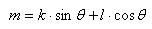
We are interested in designing a nomogram for the following equation in m, l, k and θ:
where θ > 0 and m and l lie between 0 and 100. However, the general design here is valid for other ranges of these variables.
Below is the completed nomogram, including an isopleth for the solution l = 20, m = 40, k = 50 and θ = 25°. The derivation of the design follows this figure. A high-resolution version of the nomogram can be found here.

To create this nomogram, we first draw a 100×100 grid with the origin at (0,0). The m-scale lies along the left side and increases from bottom to top. The l-scale lies on the right side and increases from top to bottom. In terms of x and y, these scales can be described by the equations (a) and (b):

The slope of the line drawn between the l and m scales can be expressed in terms of either variable:

Substituting equations (a) and (b) into (c), we arrive at

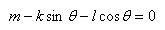
We also have the following equation that must be satisfied for this isopleth:

By substitution, equations (d) and (e) can produce independent equations for l and m:

The next step is key. These equations must be valid for any values of l and m. Therefore, if we rewrite l and m as

then l and m are arbitrary only if A=0, B=0, C=0, and D=0. Setting A=B=0 in the first equation in (f) and solving the two resulting equations for x and y provides

The same set of equations for x and y is obtained when we set C=D=0 in the second equation in (f).
Now we let k = 0, 1, 2, 10, 50, 100, 150, … and plot k-curves for the variable θ. Then we let θ = 0°, 1°, 2°, 3°, 4°, … and plot θ-curves for the variable k. This forms the nomogram shown in the figure above, which provides a linear mapping of solutions to the original equation.
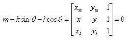
We can verify this result by substituting equations (a), (b) and (g) into the standard determinant form that describes our nomogram:

After substitution we arrive at
which is true from our original equation.
The method is equivalent to converting an equation into determinant form as
This method is generally suitable for 3, 4, 5, or 6-variable equations, but is complicated for equations of 5 or 6 variables.

It’s wonderful.I like it.Thank you Ron.
You’re quite welcome. Actually, my contribution was minor—mostly formatting the write-up to match the blog format. — Ron
LikeLike
Thanks for the details on this Liunian and Ron; some books don’t give as much explanation on grid nomograms. For example, Hall’s book (A.S Hall (1958), “Construction of graphs and charts”, London: Pitman) is unusually terse in the one example of the conversion of a four-variable relation to determinantal form, just presenting it as a fait accompli (it’s easy to verify it’s correct, but there’s not much explanation of how you’re supposed to figure out that’s what it should be). I mention Hall for no other reason than I have been rereading it in the last few days so it is fresh in my mind.
So far this is very good, but it’s clear that the nomogram needs some transformation to make the grid scale for k more evenly spaced.
There are several ways to approach this, but for me it’s easier to progress from the determinant (you’d need to write the deternimantal equation directly in terms of m.l,k and theta) and then perform projections (non-affine transformations – I can write some discussion, but it’s pretty straightforward). Hall describes a simple approach that does essentially the same thing but is more directly algebraic. Improving the k-scale in that way will make the other scales (m and l) less evenly spaced, but there’s likely to be a reasonable compromise.
It looks to me like there are no theta values above 30, in which case why do the k-curves extend past theta=30? You can’t use them beyond the last available value of theta.
This method is generally suitable for 3, 4, 5, or 6-variable equations, but is complicated for equations of 5 or 6 variables.
In general a 5 or 6 variable relation is not of the right form to be put into a nomogram. While I have seen a legitimate (i.e. for a real application) 6-variable nomogram done in grid form, usually the more variables you have the less likely you’ll be able to render it as a grid-type. Still, when it works, it’s nifty.
Thanks guys. Good stuff.
LikeLike
Hall’s book (A.S Hall (1958), “Construction of graphs and charts”
How can I get it.The graph will be changed.
LikeLike
Liunian,
I don’t know how to get it. I have seen a few copies in sales when libraries get rid of old books. It’s not unusual to find it in libraries, but I think there are better books. You may be able to get a copy online somewhere via one of the booksellers. I only mentioned Hall in particular because I was just looking at it. There are other books discuss grid nomograms, and Hall’s approach to transformation of determinantal equations (which he discusses at length for 3 variable nomograms) is simple enough that I could probably describe it for you – he essentially just adds some free parameters that represent the effect of a non-affine projective transformation, and then redraws the graph for various values of the free parameters (or sometimes after doing algebraic calculations to make things line up better).
Soreau’s book discusses them, so presumably Otto does (I don’t have Otto to hand).
Epstein has a little on grid nomograms; Hall has a little more detail than that (he at least draws a couple of diagrams).
LikeLike
Hi Glen,
The term “grid nomogram” is sometimes used for nomograms that use a grid for two variables, but still require more than one isopleth to find a solution. But you are right that there are other grid nomograms that require only one isopleth to solve equations of more than 3 variables, although there is not much discussion on them. The essay here provides, I think, a fresh and really interesting way of deriving such a nomogram without using determinants, although the determinant becomes defined in the end by substituting the variable formulas into the standard determinant form.
As you mention, Epstein has limited text and no figures on grid nomograms. In particular, he rewrites the cubic equation q^3 + uq^2 + vq + w = 0 as (q^3 + w) + uq^2 + vq = 0, which can be written in determinant form where one row depends on two variables and the other rows depend on only one variable: a11=q^3+w, a12=q^2, a13=-q, a21=-u, a22=1, a23=0, a31=v, a32=0, a33=1, which can be then reduced to standard nomographic form. The row with the two variables (the top row here in q and w) forms a grid and the other two rows are curves. This can be extended up to three rows each of two variables, giving a 6-parameter grid nomogram consisting of 3 grids. Note that when the values of x_m, y_m, x, y, x_l and y_l are substituted into the standard determinant form shown near the end of this essay, we end up with the top and bottom rows dependent on one variable each (m and l) and the middle row dependent on the other two variables (k and theta), which meets the requirement for a single-isopleth grid nomogram.
From what I can see, Soreau’s book “Contribution a la Theorie et aux Applications de la Nomographie” describes 4 such grid nomograms (Abaques LX, LXII, LXIII, and LXIV on pages 432, 437, 439 and 445). His book is in the public domain and can be found on Google Books, or downloaded from here: http://www.myreckonings.com/Temp/Contribution_a_la_theorie_et_aux_applications_de_la_nomographie.pdf . The book appears to start on page 192, but it must be an excerpt of another publication because the index indicates that the text begins on page 191. This book has a number of fascinating nomogram designs in it, actually, but I have not tried to translate the French to look into them in detail.
I believe Otto’s book also mentions grid nomograms—I will look for that. Of course, this does not detract from the unique derivation of the nomogram in the essay.
By the end of this essay we have the standard determinant form for the nomogram after we make the variable substitutions. I haven’t seen Hall’s book. Glen, if you could describe the free parameters that Hall adds to the standard determinant to transform the nomogram to more convenient forms, that would be great. You could do this by email if it’s not simple enough to post here.
Thanks,
— Ron
LikeLike
[Follow-up] Glen, Liunian and I have been corresponding on Hall’s method of transforming a nomogram by using two variables “a” and “b”. The determinant form of a nomogram can be altered to include these free variables, which can then be set to different values to transform the nomogram to a more useful layout. The variable “a” introduces a skewing (or shearing) of the scales proportional to their distance from the y-axis (or in other words, it adds a*x to the y-values in the determinant). The variable “b” changes the relative size of scale elements.
The 4-variable nomogram shown in this essay does not include all the scale lines, and in fact when they are all plotted the center grid appears much more uniform. The lines for theta-values do extend across to the y-axis, where theta=90. Also, it appeared at first to me that a shear of the k-value lines would help, as the narrowly-spaced ones at the bottom could be moved more horizontal to spread them out. However, the k-values shown in the nomogram in this essay are not equally spaced, and when they are equally-spaced a much better grid pattern is revealed. The nomogram for equally-spaced theta-values and k-values is given on the first page of this PDF file:
Click to access FourVariableNomogramShaping033008.pdf
The problem remains that as theta approaches 0, and in fact for any theta under about 30 degrees, the lines converge so much that the nomogram is very inaccurate. We would like to spread out this part of the nomogram with some kind of transformation.
The second page of the PDF file shows the changes required to a nomogram determinant to incorporate Hall’s free variables “a” and “b”, along with some examples of this nomogram when the variables are set to different values. The shearing and relative size adjustments seem to me to be most useful in “squaring-up” a nomogram to make the most effective use of the area, but the original nomogram is already square so these transformations do not appear to help so much.
We could do a projective transformation of the nomogram, which I also know Glen is very familiar with. The Projection section in this blog’s essay “The Art of Nomography III: Transformations” has a description along with a figure that I can’t reproduce here in this comment, but basically this involves a point P(x,y,z) through which all points and lines of the nomogram are projected onto the z-y plane, which then becomes the x-y plane of the new nomogram. If we place such a point P just beyond the (50,50) point where the k-lines and theta-lines converge, but a little above or below the x-y plane, then the lines near there will be spread out disproportionately as they are projected on the z-y plane. (We can’t choose a point P above or below the actual span of the grid or the points under P will be mapped to infinity.) The third page of the PDF file shows the modifications to a determinant for a projective transformation through a point P=(x_p, y_p, z_p). It also shows the transformation of this nomogram for P=(55,55,-20), which does an amazing job of spreading out the lines near the convergence. (Choosing a positive value for z_p just produces a mirror image about the y-axis of that for the negative value of z_p.)
But the l-scale and m-scale have become much smaller. And the needed height for the chart (everything below a line passing through l=0 and m=100) is also much higher than before, thus limiting any vertical enlargement that would spread out these scales. So the last page of the PDF file shows something of a compromise using P=(60,60,-30). Here the lines near the convergence are significantly spread out compared to the original nomogram, but the l-scale is not reduced as much as in the previous nomogram and the needed height for the chart is also less, allowing a greater vertical enlargement. This final nomogram seems to me to be the best choice when using central projection techniques.
This has been quite a trip! Thanks for following up with us on this, Glen, and if you or anyone reading this has any further comments or suggestions, please let us know.
— Ron
LikeLike
Hi Ron:
I don’t think you investigated what the b can do in Hall’s version. If you take your “central projection” parameters
and try b = xp/(xp – 1), you should see something similar to what you got (I didn’t work out the a that would leave that square, but I think something near a=1 or a=-1 will be right).
The zp parameter just stretches the x-scale (just makes the plot longer relative to the height).
LikeLike