Dead Reckonings

Part I of this essay described and analyzed Charles Lallemand’s L’Abaque Triomphe, the first published example of a graphical computer called a hexagonal chart. Here we discuss the mathematical principles behind hexagonal charts and provide examples of these charts from the literature of the time. The related development of triangular coordinate systems is also covered in this second part. Trilinear diagrams, a simpler offshoot of triangular coordinate systems, are still seen today in fields such as geology, physical chemistry and metallurgy (as shown to the left). A list of references is provided as well. A printer-friendly Word/PDF version with more detailed images is linked at the end, with a hexagonal overlay in the appendix that can be used to exercise these charts.

The Principles of the Hexagonal Chart

The L’Abaque Triomphe, as mentioned earlier, is an example of a hexagonal chart as invented by Lallemand in 1885. This design is sometimes referred to as an early example of a nomogram, but it only fits this description in its broadest sense. Hexagonal charts can be used to plot a function z in terms of x and y without resorting to multiple plots or a difficult-to-read 3D plot. Primarily utilized by Lallemand and Provost, hexagonal charts appear to have lived a short life as the hexagon overlay yielded to the simple straightedge used for nomograms.

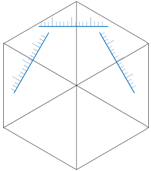
But hexagonal charts have their own charm, and in some ways they excel over nomograms. For example, today a hexagonal chart can be printed on isometric drawing paper (which has light blue lines at 0°, ±60° and sometimes 90°) or even hexagonal grid paper. Then by using the lines as visual guides there is no need to use an overlay at all! Nomograms, on the other hand, do require the use of a straightedge because the lines occur at whatever angle connects the relevant points on the scales.

The other advantages of hexagonal charts will become clearer as we look at the mathematics behind their design.

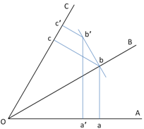
Consider the figure shown here [after Runge 1912]. Angle AOC is an arbitrary angle, but OB is a bisector of that angle. We mark points a and c such that Oa = Oc. Then we draw perpendiculars ab and cb that meet at a point on OB by the symmetry of the diagram. Then Oa = Oc = Ob cos AOB, or Oa + Oc = 2 Ob cos AOB. Now move b out to b′ on the perpendicular b-b′. Since b-b′ makes the same angles with OA and OC, aa′ = cc′, and Oa′ + Oc′ again is equal to 2 Ob cos AOB. In this way we can see that we have an addition chart where two perpendiculars from offsets a and c along OA and OC intersect along OB with an offset b of (a + b) / (2 cos AOB).

We therefore provide scales for a and c that are linear and have the same scaling factors. Then if angle AOC = 90°, the scale for their sum b will need to have a scaling factor of 1 / (2 cos 45°) = 1/√2. If AOC = 120°, the scale for their sum b is the same as the scales for a and c, since cos 60° =1/2, and this is the hexagonal chart. This property is sometimes expressed as this: the algebraic sum of the projection of a segment of a line on two axes having an angle of 120° between them is equal to the projection of the same segment onto the internal bisector of the angle between these axes. The equation then reduces to

f(b) = g(a) + h(c)

For any chosen angle AOC, an overlay is needed that provides arms perpendicular to the three scales. This is shown below for AOC = 120° (the hexagonal overlay) and for AOC = 90°, with corresponding examples shown below each of these [Werkmeister 1923]. (It’s a bit hard to make out at this resolution, but the first example shows 3 x 2 = 6 and the second example shows 3 x 5 = 15.)

If the logarithms of a, b and c are plotted along their axes, we have a multiplication rather than an addition chart, and this allows very complicated formulas to be plotted as hexagonal charts. For example, consider the formula

P = (S + 0.64)^0.58(0.74V)

Here we take logarithms of each side to express this as a simple sum.

log P = 0.58 log (S + 0.64) + log 0.74 + log V

Then we plot 0.58 log (S + 0.64) along the a scale, log V along the b scale, and log P – log 0.74 along the c scale.

Now you can see that it doesn’t matter if the scales are moved apart as long as they are shifted along an axis perpendicular to their original scale (so they are moved perpendicular to the arm of the hexagon, or in other words, parallel to their current orientation). This makes it easy to create multiple scale triplets for different ranges of the variables by placing these scales parallel to each other. With matching titles or colors, the user reads values off the appropriate triplet for the range of interest, as shown in the figure on the right.

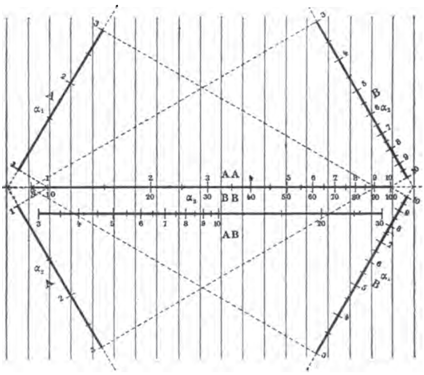
Below is an example of the use of multiple scales offset at convenient distances here and there along the 120° axes of the hexagon [d’Ocagne 1891/1899/1908/1921, Soreau 1921]. The chart is for simple multiplication of numbers, although with different labeling it could be the multiplication of functions of variables. Plotting the logarithms of the values converts the product to a simple addition. The middle scales AA, AB and BB provide the product when using scales A and A, A and B, and B and B, respectively. As examples, the intersecting dashed pair of lines at the top connect 3 on A and 3 on B, and the third vertical leg of the hexagon will terminate at 9 on the scale AB, and so forth for the other combinations shown.

Hexagonal charts can be easily extended to support the addition of four or more functions of variables. One way to do this is to group pairs of functions into grids, which we will see in later examples. This provides the value of an unknown variable with one placement of the hexagonal overlay, but is limited to three grids or six variables. Lallemand implicitly used grids when he embedded the magnetic variation effects into his maps on the chart. For simple sums such as f(a) = f(b) + f(c) + f(d), a different approach is to place the overlay to find k = f(b) + f(c) on an intermediate scale k, then slide the overlay along the arm crossing k until one of the other arms crosses f(d) on its scale, with the third arm showing the final value f(a) on that scale. This concept provides solutions for an indefinite number of summed functions, while the freedom to shift scales parallel to themselves means that the chart can be made quite compact. Later we will see an example of a tree network of hexagonal charts.

The Fate of Hexagonal Charts

Lallemand had barely publicized his highly useful invention of the hexagonal chart, originally in an internal publication of his directorate, when Maurice d’Ocagne announced his discovery of another radical means of graphical calculation, also an abaque but using what he called “parallel coordinates.” Today we call these constructions alignment charts, nomograms or nomographs.

A nomogram for the equation we considered earlier is shown in the figure on the left. A straightedge is used to cross values of S, V and P that satisfy the equation. Zooming in a bit, I get P = 1.955 for S = 2.1 and V = 1.48. The actual value of P is 1.965. Notice that there are no grid lines and no interpolating between gridlines required, a feature only possible in a hexagonal chart by using a transparent hexagon overlay. Nomograms are also indifferent to affine transformations (such as linear stretching during the printing process) and projections, which hexagonal charts are not. A survey of the field of nomography, including the derivation of this particular nomogram, can be found in several essays on this blog.

However, hexagonal charts were extensively treated even in books on nomography, as seen in the References section at the end of this essay, and work was done to create and use them in the late 1800s and early 1900s. Below are some hexagonal charts from sources contemporary to that time. Click on an image if you’d like to see a higher resolution version. A printable hexagonal overlay is found in the Appendix of the PDF file if you are interested in exercising the charts.

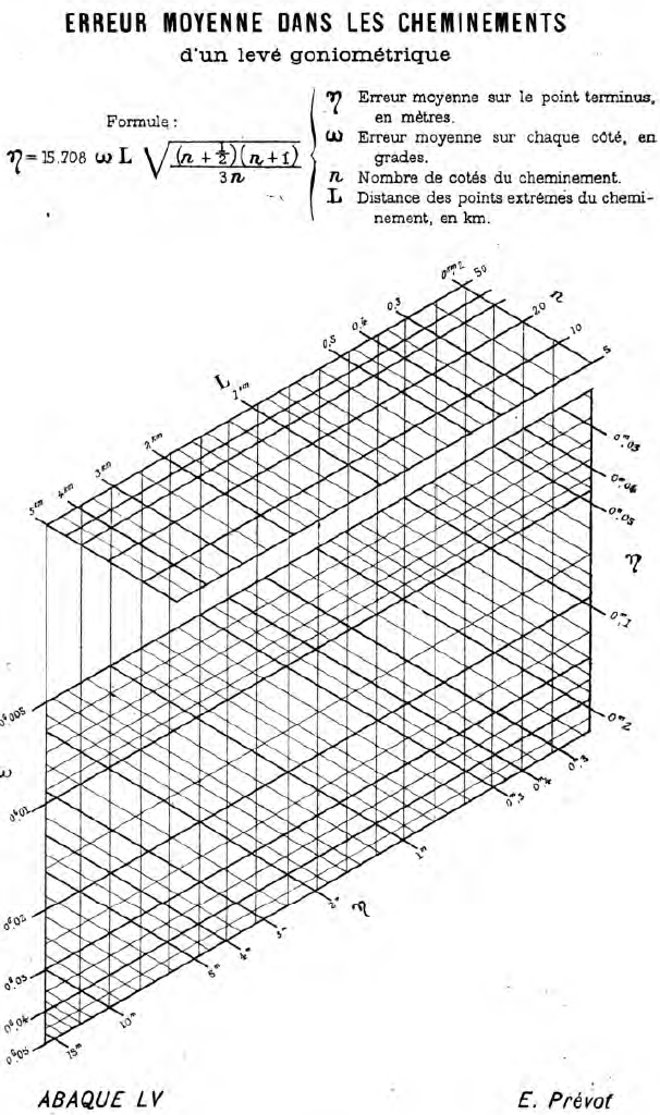
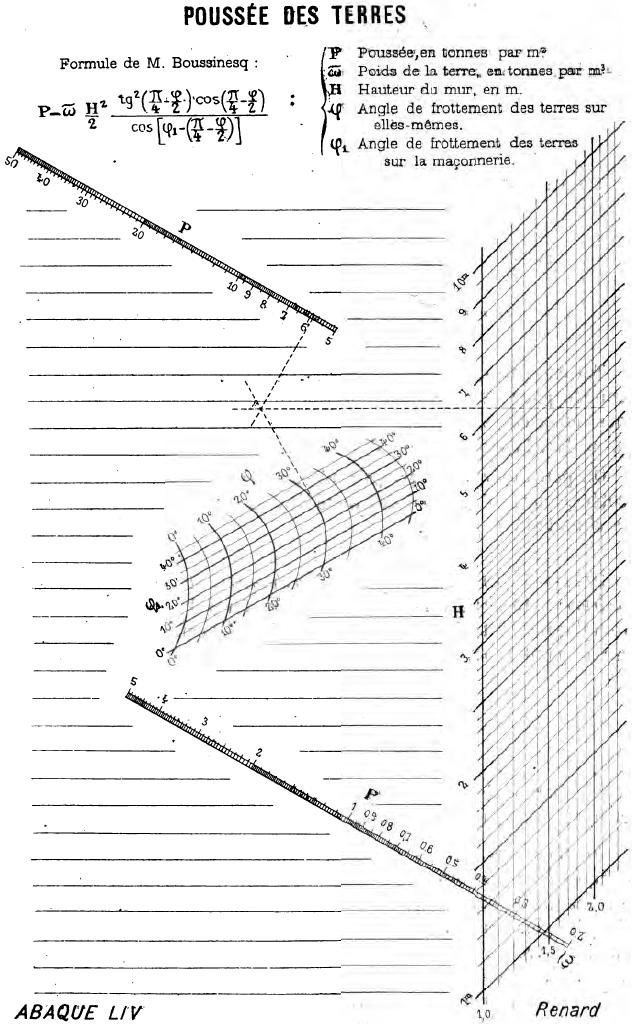
The figure below on the left is a hexagonal chart for the average error in the sighting of a level goniometer, per the equation printed along the top [Soreau 1902]. The figure on the right is a hexagonal chart for the force on the land for a vertical wall support, per the equation printed along the top of that chart [d’Ocagne 1891/1899/1921, Soreau 1902/1921].

                             

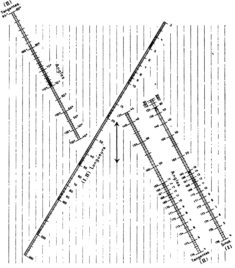
On the left below, a hexagonal chart (plotted as logarithms to convert to addition) for the Law of Sines and the corresponding tangent equation is shown, where

α₁ sin α₂ = α₄ sin α₃
α₁ tan α₂ = α₄ tan α₃

The tangent scale is split and shifted along its axis to avoid crossing the Longueurs (“Lengths”) scale for α and to maximize space on the page. A remarkable aspect of this chart is that the third scale, which would be horizontal, is missing! Here we do not need to know α₁ sin α₂ (or in this case log α₁ + log sin α₂), which would correspond to a mark along the vertical arm on the horizontal scale. Rather, we position the overlay for one set of values of α₁ and α₂ and simply slide the overlay vertically (per the arrows) to find all other values that provide the same ratio. [d’Ocagne 1899/1921].

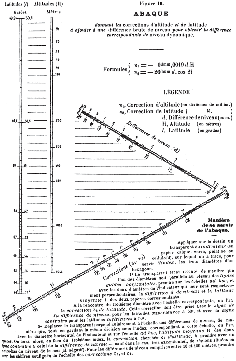
On the right below is a hexagonal abaque by Lallemand for altitude H and latitude λ corrections η₁ and η₂, respectively, based on difference in heights d [Lallemand 1889, d’Ocagne 1899/1921, Soreau 1902/1921], where

η₁ = -0.0019 d H
η₂ = -26 d cos 2 λ

                     

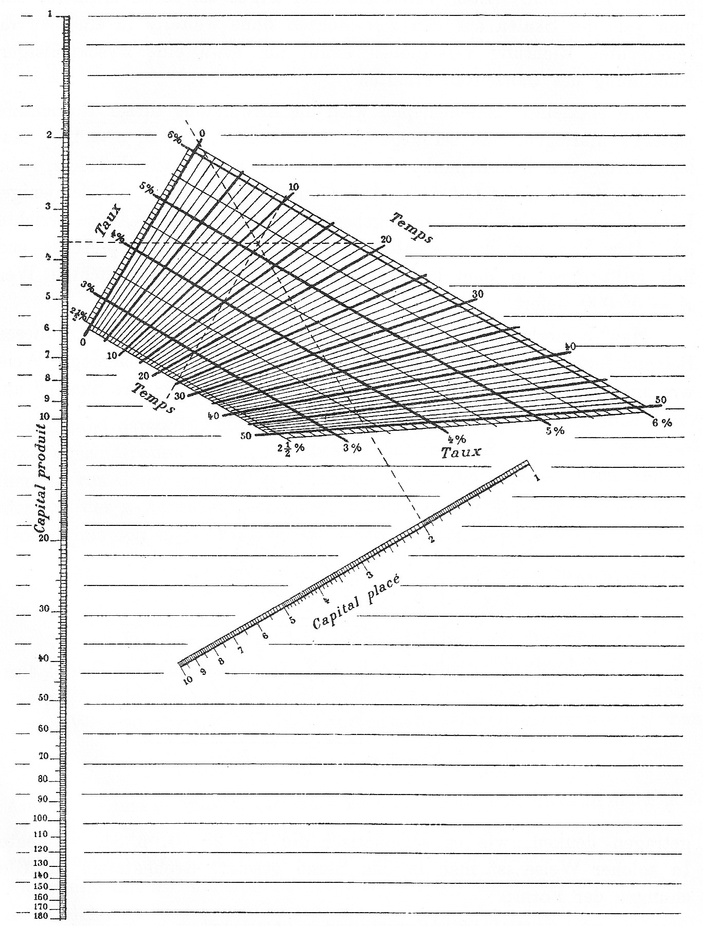
Below is a hexagonal chart for compound interest [d’Ocagne 1891/1899/1921, Schilling 1900]

A = a (1 + r)ⁿ

where:

a = Capital place
r = Taux
n = Temps
A = Capital produit

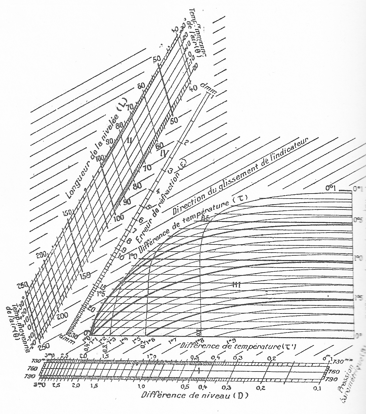
And here is a hexagonal chart for six variables (three grids) for calculating the effects of refraction. For information on the equation, see the PDF file. [Lallemand 1889, d’Ocagne 1899/1921, Soreau 1902/1921]:

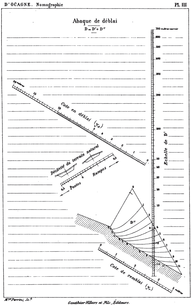
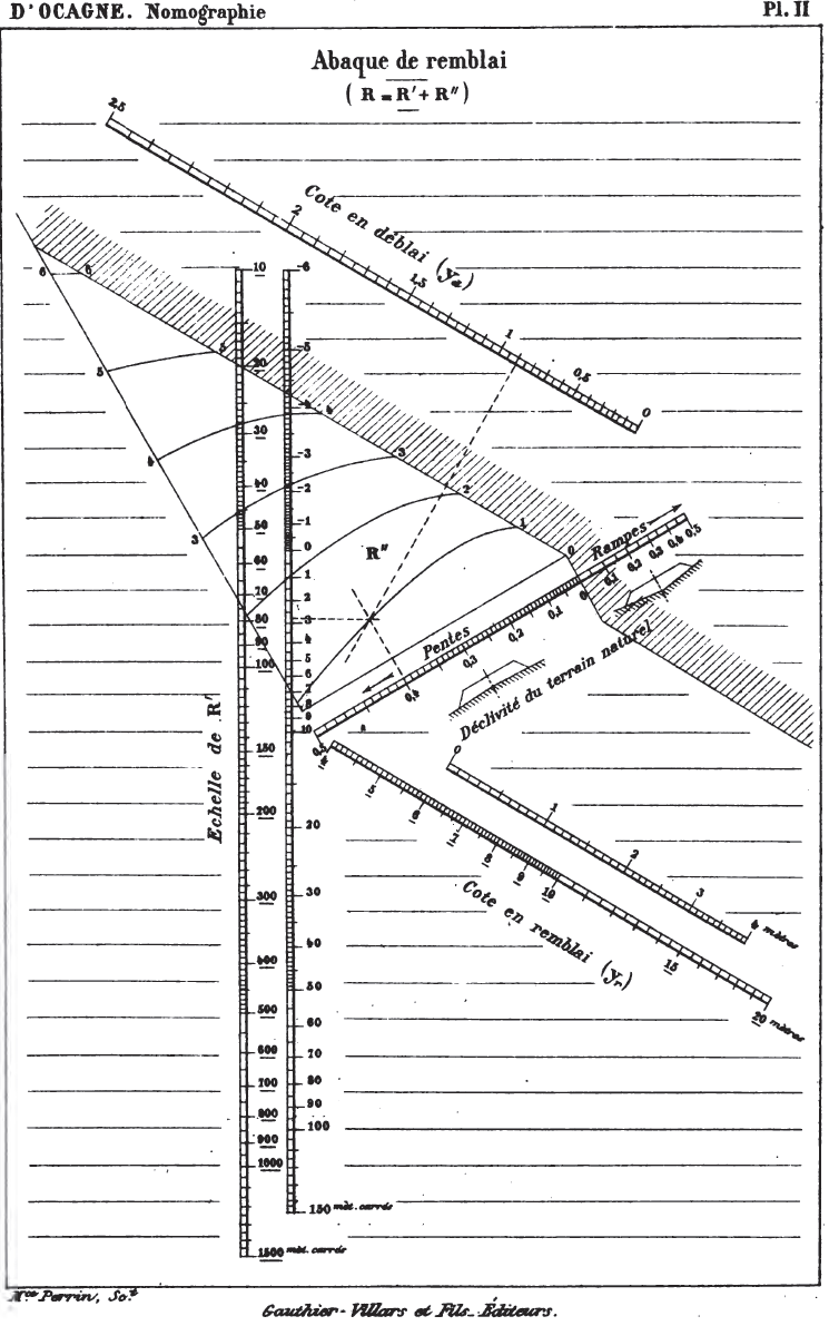
Below are two hexagonal charts for excavations and embankments, important calculations in d’Ocagne’s line of work [d’Ocagne 1899].

                

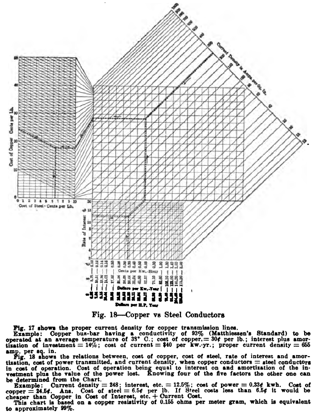
It is possible, and sometimes done even today, to compute the sum of multiple functions by chaining hexagonal charts in tree arrangements. Below is an example of such a chart [Haskell 1919].

Triangular Coordinate Systems

The ability to shift the scales also led to other graphical computers called triangular coordinate systems, and these continue in some form or other to the present day.

Consider Lallemand’s L’Abaque Triomphe. Since only the offsets from the green axes are used to align the hexagonal overlay, we can shift, say, the conical scale vertically (perpendicular to its horizontal scaling, or along the green line representing the hexagonal arm through its origin) without affecting the resulting computation. And as you can see below, if the conical scale is shifted vertically by the amount shown, the scales of the three variables can be represented along the sides of an equilateral triangle.

When three variable scales are located on the sides of an equilateral triangle, a triangular coordinate system is obtained. This is something I never encountered in school, i.e., another way of plotting a function z of two variables x and y without a 3D plot or a family of curves. As we have seen, a great number of complicated functions can be represented in this way, and with isometric or hexagonal ruled paper they are as easy to read as a 2D Cartesian plot.

Let’s return to our example of a nomogram using the same ranges as before:

P = (S + 0.64)^0.58(0.74V)

Again we take logarithms of each side to express this as a simple sum.

log P = 0.58 log (S + 0.64) + log (0.74) + log V

Below are shown two graphical calculators for this function. In the left figure, 0.58 log (S + 0.64) is plotted horizontally with a range of 1.0 to 3.5, and log V is plotted at an angle of 120° with a range of 1.0 to 2.0. Then log P – log (0.74) is plotted at 60° with a range of 1.0 to 3.4. The light blue isometric (60°) lines aid in the computation. For example, when S = 1.2 on the horizontal scale and V=1.9 on the 120° scale, the perpendiculars point to a value of P = 2.0 on the 60° scale. The actual value of P is 2.00. You have to estimate the path of perpendiculars for values that lie between the blue grid lines, but this is much easier than it first appears. And of course we can still use a hexagonal overlay for greatest precision.

In the second figure, the scales are shifted parallel to their original positions to form the triangular shape, with the 120° scale for V truncated to 1.7 so it doesn’t extend past the long 60° scale for P. However, this was for aesthetic reasons only, and it would work perfectly fine if any line extended past any other line; the only effect would be that the perpendiculars would lie mostly outside the triangle.

Let’s see, we no longer have the value V = 1.9 because of its shortened scale. Let’s try values between the grid lines, say, S = 2.1 on the horizontal scale and V = 1.48 on the 60° scale. Then I estimate P = 1.97 on the 120° scale (using the corner of a sheet of paper at the intersection of the estimated perpendiculars helps). The actual value of P is 1.965. Enlarging the figures and drawing a finer grid would provide greater accuracy. See the higher resolution versions of the left figure and the right figure.

Often in practice the sides of the triangle are moved outward and drawn longer than the scales (so the scales lie only on the portions of the sides) so that all the perpendiculars, or at least the perpendiculars for the ranges of interest, lie inside the triangle. The example on the right is from Otto [1963].

Fasal [1968] provides a derivation of the general case of an acute triangular coordinate system of three unique angles. This general equation is

g(y) = k₁f(x) + k₂h(z)

where k₁ = cos β / cos α and k₂ = sin (α+β) / cos α when f(x), g(y) and h(z) have identical scaling. It can be seen from the figure that the three angles of the triangle are α+β, 90°- α and 90°- β. Fasal provides a graphical way of choosing these internal angles of the triangular coordinate system for given ranges of the variables in order to minimize the overhang of the scales beyond the vertices of the triangle. Aiken [1937] also discusses these relations in a very readable paper.

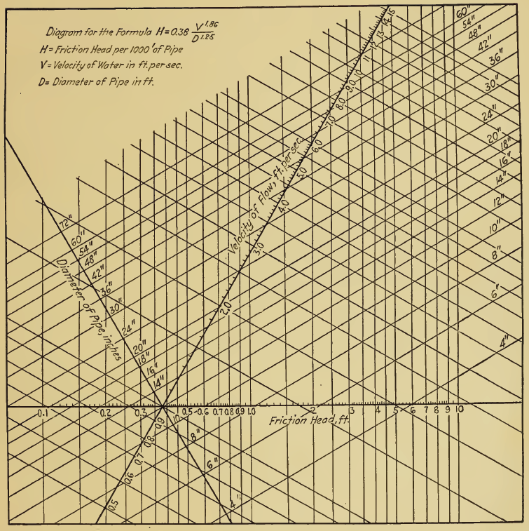
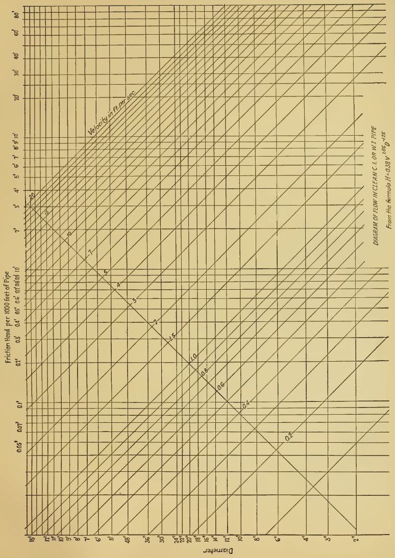
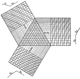
Shown here are two different graphical representations for the friction head H in feet per 1000 feet of water of water flowing in a pipe of diameter d with a velocity of V feet per second [Hewes 1923]:

H = 0.38 V^1.86 / d^1.25

The first figure shows this function plotted in on hexagonal axes, where the solution can be found with using the grid or with a traditional hexagonal overlay. The second figure shows the same function plotted in a triangular coordinate system. Click on them to see higher resolution versions.

The figure below shows a triangular coordinate system where the triangle has been trimmed to save space, which therefore requires that the scales be chopped into two parts apiece [Lacmann 1923]. The equation represented by this chart is

v = 43.1 d ^0.62 J^0.55

 
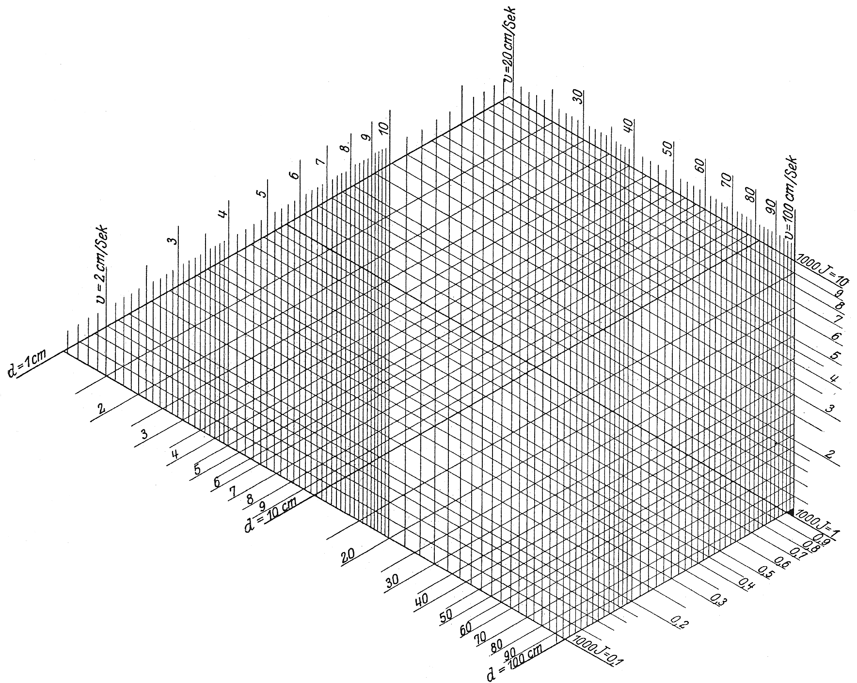
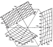
Now it’s also possible to map the scales of a hexagonal chart onto the sides of an equilateral triangle as shown in the figure on the right, where the three scales (or in this case, three grids) are mapped onto the sides of the triangle [Lacmann 1923]. Note that here the guidelines are parallel to the sides rather than perpendicular to them. A hexagonal overlay with its center inside the triangle can align its arms to the three sides of the triangle. Based on the workings of a hexagonal overlay, you can see that for a triangle with equally-spaced scales along each edge, the line segments from any node in the middle of the triangle will terminate at three scale values that add to a fixed value. This construction is called a trilinear chart or trilinear diagram.

Below is a three-variable equation constructed as a trilinear chart. The fixed sum can be readily seen as the sum at any vertex of the triangle, such as the (100+0) sum at the lower corners. The upper vertex is the same except that v²/2g is plotted so you would have to perform the inverse to find 100 along the right scale at the vertex. This is a triangular coordinate system for solving Bernoulli’s Equation for incompressible flow [Lacmann 1923]. Click on it to see a higher resolution version.

z + p/γ + v²/2g = 100

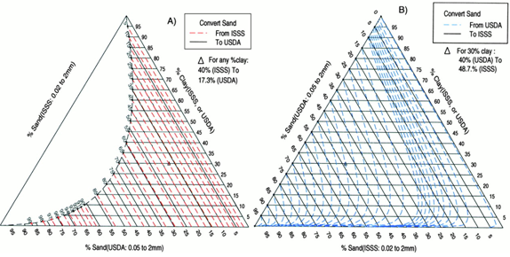
Trilinear charts are actually in use today, generally for finding the result of mixing three components (such as gases, chemical compounds, soil, color, etc.) that add to 100% of a quantity. These usually have percents of each component listed on the three scales along the sides of the triangle, as shown in the first figure below [Newski 1955].

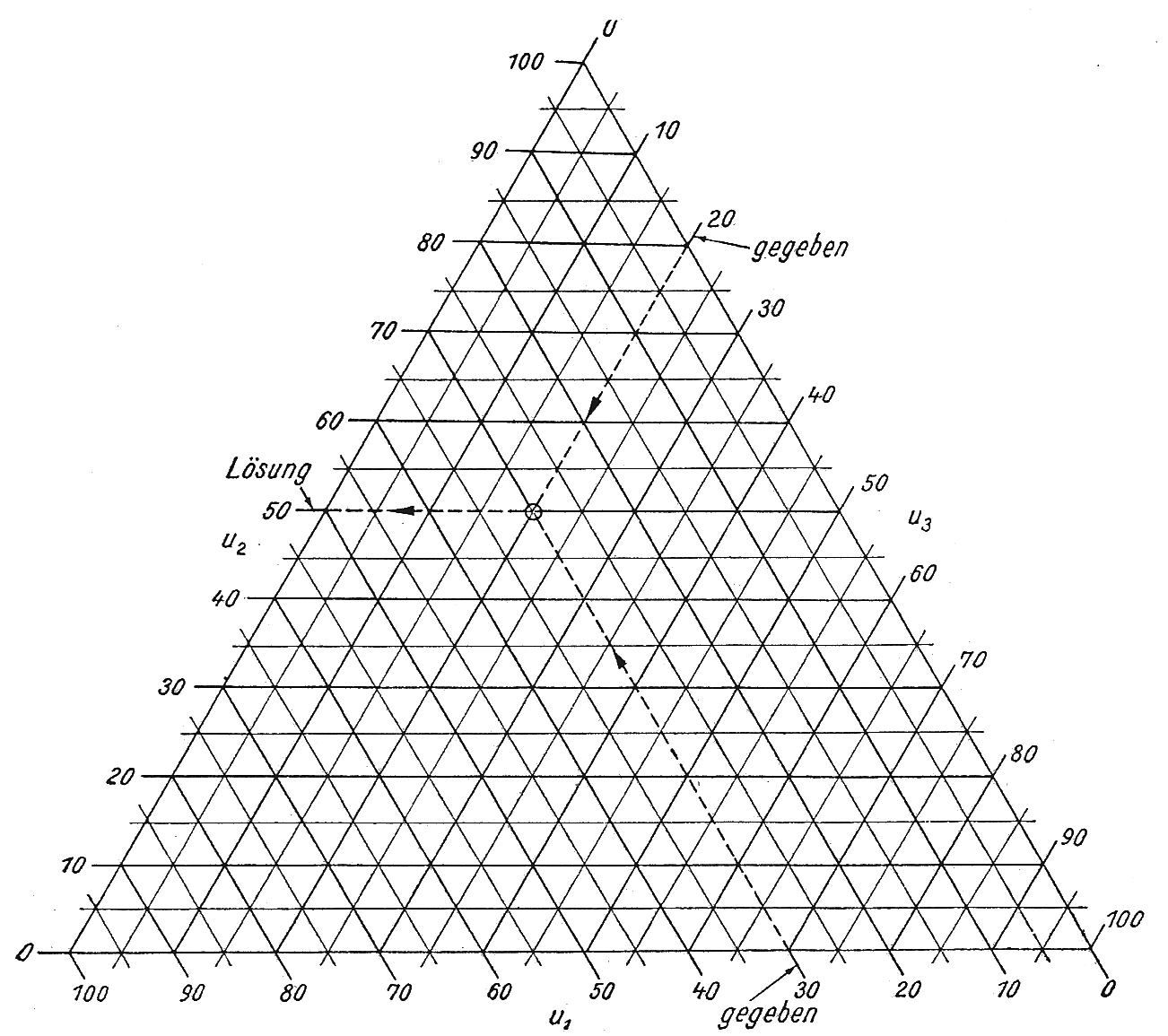
By itself there is not much information here, but it is possible to add a fourth variable as contour lines within the triangle, as in the figure above. For example, variations in the percentages of metals in an alloy result in different hardness, brittleness, etc. The user can select a mixture whose node lies on the contour line for the desired attribute. This is equivalent to having curves in the middle of a hexagonal chart for the center point of the overlay as seen in the figure to the right [Soreau 1921].

J. Williard Gibbs is credited with the first use of trilinear coordinates (for thermodynamics) in 1873 [Howarth 1996]. In 1881 Robert Thurston published a paper using trilinear coordinates to express the properties of copper-zinc-tin alloys using contours [Aiken 1937]. Therefore, it seems likely that these constructions preceded hexagonal charts, and perhaps Lallemand drew inspiration from them. In any event, trilinear graphs exist today for the same types of applications. The Piper trilinear diagram, for example, is used to plot measured values of concentrations of major ions in samples of ground water onto an array of such triangles.

The trinary diagram below was published by S. F. Taylor in 1897 to graph the critical curve (the solid line) and tie-lines (the broken lines) between five conjugate pairs of compositions (I-VI) of a benzene-water-alcohol system. The crosses represent experimental data [Howarth 1996].

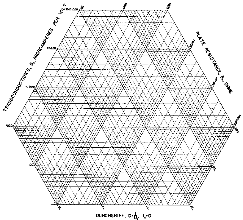
The figure below shows an equilateral triangular coordinate system with truncated corners to characterize vacuum tubes. The logarithmic scale values that would have been along the removed sections are simply wrapped around the edges of the truncated sections [Aiken 1937]. Click on it to see a higher resolution version.

A Whisper of the Past

Hexagonal charts share an interesting legacy with their triangular cousins. Today we don’t see hexagonal charts at all, partly due to the need for a hexagonal overlay. Triangular coordinate systems are also rare with the exception of the easily plotted and readily-understood trilinear diagram. Graphical constructions based on intersections of lines and curves on a Cartesian x-y coordinate system (intercept charts or lattice charts) are sometimes encountered, as in phase diagrams of thermodynamics. Hexagonal charts filled a relatively brief need for a graphical calculator prior to the invention of nomograms, which in turn fell victim to the development of calculators and computers. The study of these developments, so treasured at the time and so overlooked today, evokes a real appreciation, at least in me, of the ingenuity and pressing human efforts that were made in the past. I can sense a real purpose, and sometimes a surprising turn of imagination, in the writings of these individuals.

References

NOTE : The references with Google Books links are fully viewable and downloadable within the United States, but not necessarily in other countries due to variations in copyright laws.

Aiken, Howard. 1937. Trilinear Coordinates. Journal of Applied Physics, 8:470-472. Available for download with IEEE Xplore access such as in university libraries.

d’Ocagne, Maurice. 1908. Calcul Graphique et Nomographie. Paris: Gauthier-Villars. Available for download.

d’Ocagne, Maurice. 1891. Nomographie; les Calculs usuels effectués au moyen des abaque. Paris: Gauthier-Villars. Available for download.

d’Ocagne, Maurice. 1899. Traité de nomographie. Paris: Gauthier-Villars. Available for download.

d’Ocagne, Maurice. 1921. Traité de nomographie. 2nd Ed. Paris: Gauthier-Villars.

Fasal, J. H. 1968. Nomography. New York: Ungar.

French, Thomas E. and Vierck, Charles J. 1958. Graphic Science; Engineering Drawing, Descriptive Geometry, Graphical Solutions. New York: McGraw-Hill.

Haskell, Allen C. 1919. How to Make and Use Graphic Charts. New York: Codex. Available for download.

Hewes, Laurence J. and Seward, Herbert L. 1923. The Design of Diagrams For Engineering Formulas And the Theory Of Nomography. New York, McGraw-Hill. Available for download.

Howarth, Richard J. 1996. Sources for a History of the Ternary Diagram. The British Journal for the History of Science, Vol. 29, No. 3. Available for download with JSTOR access.

Lacmann, Otto. 1923. Die Herstellung gezeichneter Rechentafeln: Ein Lehrbuch der Nomographie. Berlin: Verlag von Julius Springer.

Lallemand, Charles. 1885. Les abaques hexagonaux: Nouvelle méthode générale de calcul graphique, avec de nombreux exemples d’application. Paris: Ministère des travaux publics, Comité du nivellement général de la France.

Lallemand, Charles. 1889. Nivellement de Haute Précision, in Lever des Plans et Nivellement. Paris: Librairie Polytechnique. Available for download.

Lipka, Joseph. 1918. Graphical and Mechanical Computation. New York : John Wiley & Sons. Available (in a 1921 volume) for download.

Newski, B. A. 1955. Prakitum der Nomogramm-Konstructionen. Berlin: Akademie-Verlag.

Otto, Edward. 1963. Nomography. New York: Macmillan.

Peddle, John B. 1919. The Construction of Graphical Charts. New York: McGraw-Hill. Available for download.

Runge, Carl. 1912. Graphical Methods. New York : Columbia University Press. Available for download.

Schilling, Friedrich. 1900. Ǖber die Nomographie von M. d’Ocagne. Leipzig: Druck und Verlag von B. G. Teubner. Available for download.

Shirazi, Mostafa, et. al. 2001. Particle-Size Distributions: Comparing Texture Systems, Adding Rock, and Predicting Soil Properties. Soil Sci. Soc. Am. J. 65:300–310.

Soreau, Rodolphe. 1902. Contribution á la théorie et aux applications de la nomographie. Paris: Ch. Bèranger. Available for download.

Soreau, Rodolphe. 1921. Nomographie ou Traité des Abaques, Paris: Chiron.

Werkmeister, P. 1923. Das Entwerfen von graphischen Rechentafeln (Nomographie). Berlin Verlag von Julius Springer.

<<< Go to Part I of this essay
Highest Resolution and printer-friendly Word file of Lallemand’s L’Abaque Triomphe, Hexagonal Charts, and Triangular Coordinate Systems Parts I-II

Printer-friendly PDF file of Lallemand’s L’Abaque Triomphe, Hexagonal Charts, and Triangular Coordinate Systems Parts I-II