Dead Reckonings

Those of us who enjoy our expeditions through the lost world of nomography quickly discover that many original sources that are still considered masterpieces in the field have never been translated into English. In my case this is a serious handicap, and I find myself struggling through the texts trying to understand the rationale behind the beautiful nomograms I see on the printed page. Nomography and its predecessors were invented in France and only later spread to such places as Germany, the U.S, Britain, Russia and Poland. Today it seems to me that most research appears in Czech journals. In addition to the language difficulties, many of the original sources are in obscure, hard-to-find journals.

In 1982 H.A. Evesham produced his doctoral thesis, a review of the important discoveries in nomography. It is often cited in other works, but unless you know someone who knows someone, it is very difficult to find—I have never been able to locate a copy. However, just recently Mr. Evesham’s thesis has been professionally typeset and released as a book (click here or here) by Docent Press under the aegis of Scott Guthery. If you have an interest in the theoretical aspects of nomography beyond the basic construction techniques of most books and of my earlier essays, you will appreciate this book as much as I do. Mr. Evesham does a wonderful job of weaving mathematical discoveries in nomography from many contributors into a readable but scholarly work.

This is a book about the theory of nomography—there are mathematical derivations and sketches of the corresponding scale curves, but few finished nomograms. The mathematics presented here are tools that can be extremely useful in designing your own nomograms, and in fact the nomograms presented in this review were made by me using Leif Roschier’s PyNomo software. (If you haven’t read anything about nomograms yet, please see this essay or this article.)

Two major threads in the history of nomography are existence criteria and anamorphosis. Existence criteria can tell you if the equation you are interested in can be represented as a nomogram (i.e., can be expressed as a determinant equation in standard nomographic form). It provides guidance in algebraically converting your equation to one of the canonical forms that have matching nomographic forms. This process generally involves derivatives, so some basic knowledge of how to take a derivative or find an integral (or simply a book of tables of these) is needed to really test your equation. Anamorphosis is the process of manipulating your equation into different forms of nomograms, say from three parallel scales to one curve containing two scales and one line, or even a single curve along which all three scales lie. It is more than simple geometric transformations or projections.

A brief overview of the history of nomography is given in a later paper by Evesham; the thesis, of course, goes into much greater mathematical detail. Evesham first describes the work of Leon Lalanne, who in 1843 adjusted the x and y axis scaling on a Cartesian plot to morph the curves for the equation xy = k into straight lines. In the process he created the first log-log plot in history and ultimately produced his “Universal Calculator” graphical computer seen on the cover of Evesham’s book. I have been meaning to write an essay on this calculator for some time. Lalanne is the one who termed this process anamorphosis.

The road from Lalanne to d’Ocagne’s invention of nomography strikes me as a strange one, a slow trip until 1867, and then an explosion of ideas in the 1880s. The event in 1867 was Paul de Saint-Robert’s presentation of his test to determine if an equation can be represented by two fixed scales and a sliding scale (like a special slide rule). This is equivalent to the three parallel scales of d’Ocagne’s later nomogram for simple addition of three functions. In other words, we are interested in whether an equation in the form F(x,y,z) = 0 can be rewritten in the form Z(z) = X(x) + Y(y). The Saint-Robert criterion says this is possible if

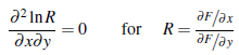
where the partial derivative ∂F/∂x is the derivative of F with respect to x assuming all other variables are constants, and ∂F/∂y is the derivative of F with respect to y assuming all other variables are constants. To find ∂² ln R / ∂x∂y, we find the partial derivative of ln R with respect to x and then we find the partial derivative of the result with respect to y.

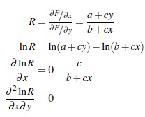
Let’s see if this works. Say we want to create a nomogram for the equation z = ax + by + cxy + d, or F(x,y,z) = –z + ax + by + cxy + d = 0. I created a nomogram last summer for this equation for an upcoming blog essay on nomograms to model 2-, 3- and 4-factor linear equations in Design of Experiments (DOE) methodology; this equation is the general form for a weighted, linear 2-factor equation. Can we draw it as three parallel scales in x, y and z? Here,

So yes, we find that we can create a simple addition nomogram of three parallel scales as Z(z) = X(x) + Y(y). Saint-Robert also provides a way of finding the functions X(x), Y(y) and Z(z) to plot on the scales:

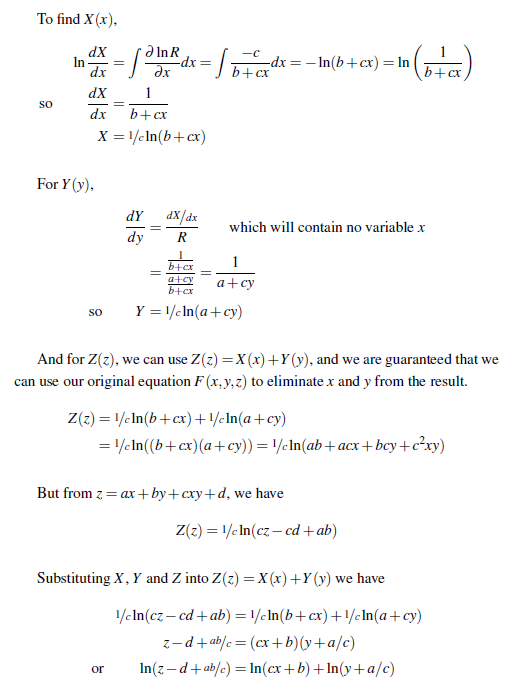
which in the logarithmic form is the correct addition form for the parallel-scale nomogram, where the functions on the z, x and y scales are given by the corresponding terms Z(z), X(x) and Y(y). This nomogram is shown below for the specific equation z = 5x + 10y + 2xy. The sample isopleth (index line) demonstrates the graphical calculation of z=150 when x=2 and y=10. Click on this figure and all figures in this essay for full-resolution versions.

 

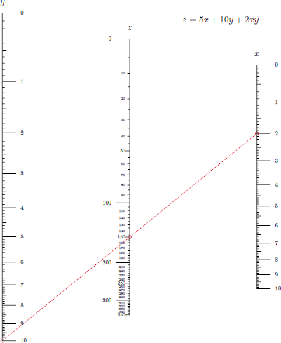
So you might say, well, I could have figured out that z = ax + by + cxy + d can be written as z – d – ab/c = (cx + b) (y + a/c) without going through all this. In my case, I didn’t realize it was generally possible when I was creating the nomogram, and it took some painful transformations of the nomogram I originally created to arrive at this parallel-scale form. Only then did I think to algebraically derive it. Doh!

Saint-Robert’s criterion is also useful for more complicated equations for which it is difficult to determine if a simple addition form exists. For example, an equation of the form

can be cast as

In fact, the variables x, y and z can be replaced here by any function f₁(x), f₂(y) and f₃(z) and this formulation holds. I’ve written out the complete derivation for this example using Saint-Robert’s criterion that you can find here.

Evesham also describes two different criteria by Massau and Lecornu for expressing F(x,y,z) = 0 in the form Z₁(z)X(x) + Z₂(z)Y(y) = 1, which is equivalent to the general form Z₁(z)X(x) + Z₂(z)Y(y) + Z₃(z) = 0 after division by Z₃(z).

Evesham continues his presentation by discussing the important existence theorems of Grönwall, Kellogg and Džems-Levi. Ultimately he points to Warmus’ publication Nomographic Functions in 1959 as the first comprehensive treatment of existence criteria for functions of three variables. Warmus uses exhausting algebraic techniques based on classifications of equations to either find the determinant elements or show that it is not possible. Thank goodness it’s written in English despite being published in Rozpravy Matematyczne. I have this little book, but it’s one that I have no plans to read through until I really need to.

An overview of d’Ocagne’s Traitè de Nomographie of 1899 (found at Google Books and as modern facsimiles 1 and 2 on Amazon) is provided. This is followed by a detailed look at J. Clark’s nomographic discoveries. I found this particularly exciting, as d’Ocagne, Soreau and others include Clark’s nomograms in their books and they discuss his methods of anamorphosis, but I had never found any book authored by Clark. In fact, I learned that Clark instead authored in 1907-1908 a series of articles on nomography in a French mechanical engineering journal, which to my surprise I subsequently found digitized at Google Books (see pages 321-335 and 575-585 of here and pages 238-263 and 451-472 of here).

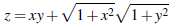
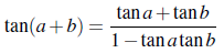
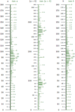
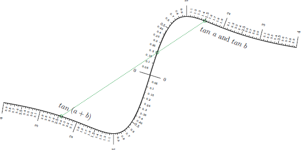
Let’s take a look at some of Clark’s ideas discussed in Evesham’s book. We’ll use an equation that Clark used, the addition formula for the tangent function:

As Soreau points out, this can actually be drawn as a basic parallel scale addition nomogram. In one approach that I can only call inspired, you first create a nomogram for (a+b) = a + b, which for a parallel-scale nomogram consists of identical linear scales for a and b and a linear scale for (a+b) with half the spacing of the other scales and located exactly between them. Then you just plot the tangent of each value on the other side of the scales, and (voila!) you have an addition nomogram for the tangent function. A straightedge (isopleth) placed across the values on the tan a and tan b scales will cross the corresponding value on the tan (a+b) scale.

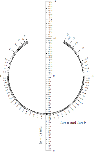
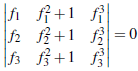
Clark looked at what nomographic forms are possible with given orders of equations. One of his results is that an equation in the form f₁f₂A₃ + (f₁ + f₂)B₃ + C₃ = 0 can be represented by the following general determinant equation:

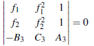
where A₃, B₃ and C₃ are functions of the third variable. If you actually multiply out the determinant you will get the equation (f₂ – f₁)[f₁f₂A₃ + (f₁ + f₂)B₃ + C₃] = 0 which satisfies the original equation but consists of an extra factor (f₂ – f₁). More on that later!

With the substitution f₁ = tan a, f₂ = tan b and f₃ = tan(a+b), the tangent addition formula can be written as

f₃ = (f₁ + f₂) / (1 – f₁f₂)     or      f₁f₂f₃ + f₁ + f₂ – f₃ = 0

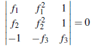
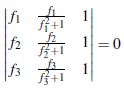
If we match this to Clark’s form above, we find that A₃ = f₃, B₃ = 1 and C₃ = -f₃ so the determinant equation is of the form

And dividing the third row by f₃ we arrive at the standard nomographic form:

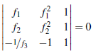
When a nomogram is in this standard form, the first two columns are the x and y functions for the scales for each variable, so you can see that the scale for tan a lies on a parabola (since x = tan a and y = tan²a means that y = x²), and the tan b scale lies on exactly the same curve. The tan(a+b) scale lies on the line y = -1. A straightedge (isopleth) is placed across the value of tan a and the value of tan b on the parabola, and tan(a+b) will be the value crossed on the linear scale.

 

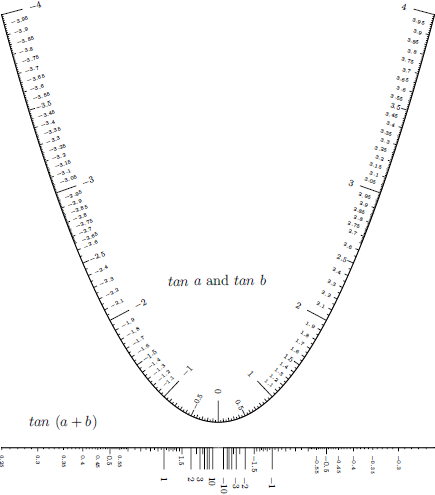
Clark calls this a conical nomogram, and it’s very interesting that two of the three scales lie on the same curve, although if f₁ and f₂ are not the same function the scale labels will be different (and therefore usually printed on opposite sides of the curve). Evesham provides examples for the equation f₁ + f₂ = f₃ and f₁f₂ = f₃ expressed in Clark’s form.

Evesham also mentions that a homographic transformation can always transform this parabola into another conic such as a circle. A circle is far easier to draw by hand, and I think it provides a very striking nomogram. Evesham does not explain how this is done. I had in fact converted a hyperbolic scale to a circle previously in my nomography essays but it was a multi-step process, so I went to Clark’s original articles on Google Books and found his method for doing this transformation (on page 262 here).

For Clark’s general determinant equation given above, a circle will result if the elements of the determinant are replaced with the functions below:

(Note that Clark uses columns 2 and 3 in his articles for the x- and y-elements, but I’ve moved them to the more standard columns 1 and 2 in the determinant above.)

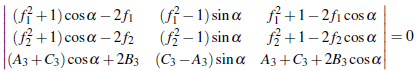
We can choose the angle α, and in fact this positions the opening of the parabola on the circle. We can’t choose α = 0 here because sin α = 0 and so the y-elements are 0. If we choose α= 45° we get the nomogram below, where the opening is at this 45° angle:

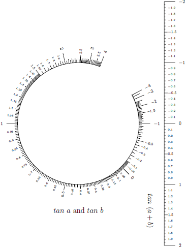
The circular scale is compressed asymmetrically, but if we get the figure below if we choose α = 89.99° (we can’t choose 90° or the row 3, column 3 element is 0 since A₃ = -C₃ and we can’t divide that row by any number to get the determinant in standard form):

The thing that Clark did that is most astonishing to me is to find a way to generalize his equation form and provide a means of getting all three scales to lie along a single curve! Clark deduced that the extraneous factor (f₁ – f₂) in the determinant for the conical determinant is responsible for aligning two of the three scales (f₁ and f₂ here but we can use any two of the variables) on a common curve, so he searched for a factor that would align all three scales. For an equation in the general form

f₁f₂f₃ + A(f₁f₂ + f₂f₃ + f₁f₃) + B(f₁ + f₂ + f₃) + C = 0           (1)

he found that the extraneous factor should be (f₁ – f₂)(f₂ – f₃)(f₃ – f₁), and this leads to the determinant equation:

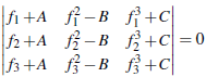
You can see from the x- and y-elements of each row that the three scales lie on exactly the same curve, although if the functions are not identical the scale divisions will be different.

So let’s see, we can rewrite the tangent addition formula as f₁f₂f₃ – (f₁ + f₂ + f₃) = 0 for f₁ = tan a, f₂ = tan b and f₃ = -tan(a+b). Matching terms with the general form above, we find that A = 0, B = -1 and C = 0, so the determinant equation is:

Now we can add the first column to the third, divide by the second column, and shift the first column to the third column to get this into standard nomographic form:

For f₁ = tan a, the scale curve is given as x = tan a, y = tan a / (tan²(a) + 1) and the same for f₂ = tan b and f₃ = tan(a+b) and we have this remarkable nomogram below for tangent addition, which Clark termed the acnodal form:

 

In fact, the general equation form breaks into three distinct nomographic curve types that cannot be transformed into each other, represented by the following forms:

f₁f₂f₃ = 1 (crunodal form)
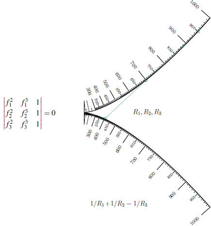
1/f₁ + 1/f₂ + 1/f₃ = 0 (cuspidal form)
f₁f₂f₃ – (f₁ + f₂ + f₃) = 0 (acnodal form)

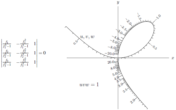
We have just seen the general acnodal form in our tangent addition nomogram. You may have seen the crunodal form below in my other essays or nomography calendar. This curve is also known as the folium of Descartes. The equation  f₁f₂f₃ = 1 corresponds to A=0, B=0 and C=-1 in Clark’s general equation (1) given above:

The cuspidal form is used for the harmonic relation, which can represent, for example, the focal length of two lenses in series or the equivalent resistance of two resistors in parallel: 1/f₃ = 1/f₁ + 1/f₂. This can be written as  1/f₁ + 1/f₂ + 1/(-f₃) = 0 to get it into our form above. It’s not very practical for graphical calculation as you can see from the example below of 1/950 + 1/700 = 1/403, but it’s a very interesting nomogram nonetheless. The equation  1/f₁ + 1/f₂ + 1/f₃ corresponds to A=1, B=0 and C=-f₁f₂f₃ in Clark’s general equation (1) given above, because you can rewrite 1/f₁ + 1/f₂ + 1/f₃ as (f₁f₂f₃)^-1 (f₁f₂ + f₂f₃ + f₁f₃). With work you can find this determinant equation and its corresponding nomogram:

Actually, it’s possible to find a single curve nomogram for f₁ + f₂ + f₃ = 0 as well, as shown below. Another way of looking at this is that the 3 real roots of a cubic equation ax³+bx²+cx+d = 0 sum to –b/a, so a plot of y = x³ marked with its x-values provides a single scale nomogram for addition:

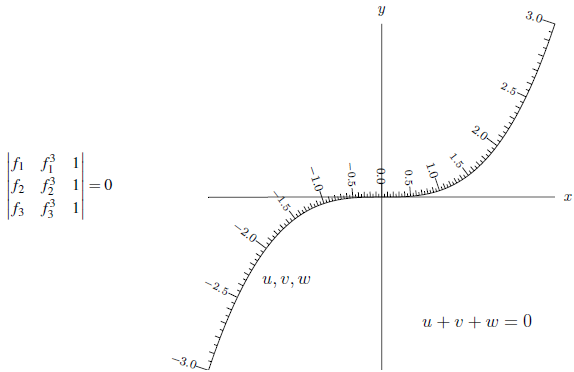
Clark called all of these cubic forms of nomograms because the common curve in each case is given by a third-degree equation.

Evesham concludes his thesis with a discussion of Russian advances in nomography from the 1950s, including the use of oriented transparencies of scales laid across other printed scales as treated by Khovanskii. This type of nomogram can incorporate more variables in a single alignment. He refers to earlier work by Margoulis, and I have Margoulis’ book, Les Abaques à transparent orienté ou tournant, from 1931 that includes extremely interesting nomograms for aeronautics (such as attack angles for helicopters!), and which uses oriented transparencies to solve very complicated equations of several variables.

H.A. Evesham’s thesis weaves together many different threads in the history of nomographic theory. If the presentation above intrigues you, then you will find real treasures in this book. The bibliography in the book is valuable in itself for searching out more details. I enjoyed reading the book immensely. Mr. Evesham does a great service in making these advancements available to those of us today with an interest in the field of graphical calculation. Again, the book can be found here or here.

(I have no financial interest in the book.)