Dead Reckonings

In 1885, Charles Lallemand, director general of the geodetic measurement of altitudes throughout France, published a graphical calculator for determining compass course corrections for the ship, Le Triomphe. It is a stunning piece of work, combining measured values of magnetic variation around the world with eight magnetic parameters of the ship also measured experimentally, all into a very complicated formula for magnetic deviation calculable with a single diagram plus a transparent overlay. This chart has appeared in a number of works as an archetype of graphic design (e.g., The Handbook of Data Visualization) or as the quintessential example of a little-known graphical technique that preceded and influenced d’Ocagne’s invention of nomograms—the hexagonal chart invented by Lallemand himself. Here we will have a look at the use and design of this interesting piece of mathematics history, as well as its natural extension to graphical calculators based on triangular coordinate systems. Part I of this essay covers Lallemand’s L’Abaque Triomphe, while Part II covers the general theory of hexagonal charts and triangular coordinate systems. A printer-friendly Word/PDF version with more detailed images is linked at the end of the essay.

As an engineer Lallemand (1857-1928) [1, 2] created a number of ingenious devices to assist in determining altitudes, water and tides in France involving water levels, mercury baths, air bubbles, and other gauge techniques. Slow changes in these measurements led him to theoretical investigations of lunar tides in the Earth’s crust. He also created the modified polyconic form of map projection. Maurice d’Ocagne was his deputy from 1891 to 1901; his indebtedness to Lallemand is evident in his detailed treatment of hexagonal charts and his brief description of L’Abaque Triomphe in his masterpiece Traité de Nomographie and other works on nomography and its foundations [d’Ocagne 1891/1889/1921, Soreau 1902/1921].

What is Magnetic Deviation?

A well-constructed compass on a ship will fail to point to true (geographic) north due of two factors:

---

Magnetic variation (or magnetic declination): the angle between magnetic north and true north based on local direction of the Earth’s magnetic field, and

Magnetic deviation: the angle between the ship compass needle and magnetic north due to iron within the ship itself.

---

Magnetic variation has been mapped over most of the world since the year 1700, although it changes over time due to drifting of the magnetic poles of the Earth. The compass correction for magnetic variation can be made based on published magnetic variation tables.

Magnetic deviation arises from the magnetic effects of both hard and soft iron in the ship. Hard iron possesses permanent magnetism as well as semi-permanent magnetism imprinted by the Earth’s magnetic field under the pounding of the iron during the ship’s construction, or from traveling long distances in the same direction under the influence of this field. Collisions, lightning strikes and time will cause significant changes in this magnetism. External fields such as the Earth’s magnetic field induce magnetism in soft iron in the ship on a near real-time basis, an effect that varies with location as the Earth’s magnetic field varies in strength and direction. The combination of magnetic fields from the iron of a particular ship produces a magnetic field that affects the accuracy of compasses onboard that ship, sometimes dramatically. A detailed account of the origins and history of magnetic deviation can be found in another essay of mine.

The Equations of Magnetic Deviation

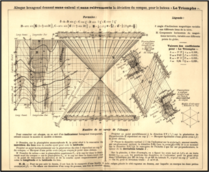
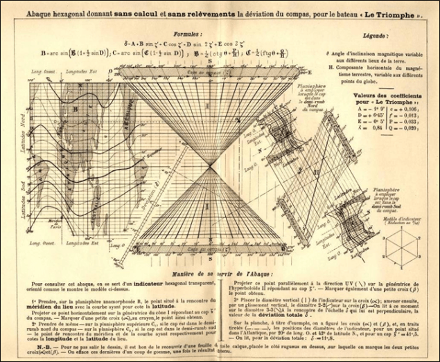
Lallemand’s L’Abaque Triomphe is shown below (a high-resolution version is also available). It provides a graphical means (an abaque) for calculating the magnetic deviation of the ship Le Triomphe for a given compass course and location on Earth using equations developed by Archibald Smith in 1843. The magnetic deviation essay mentioned above provides the background and analysis of these equations (where the mathematical derivation is given by a hyperlink in the online version of the essay and in the Appendix of the PDF version hyperlinked at the end of the webpage).

The magnetic deviation equations use both non-bold and bold variables A, B, C, D and E, as well as measured magnetic parameters of the ship. Here the angle ξ′ is the compass course, or the angle from north indicated by the compass needle, and δ is the magnetic deviation, or the angle correction to be applied to the compass course to counteract the effects of magnetic deviation.

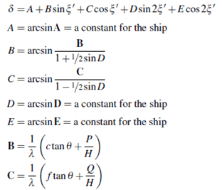
where at a given location of the ship,

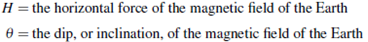
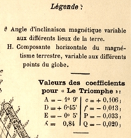
and A, D, E, λ, c, P, f and Q are parameters deduced for a particular ship. These formulas assume a magnetic deviation of less than about 20° in order that B and C can be expressed as simple arcsine functions, and so a certain amount of correction for magnetic deviation may be needed in the binnacle holding the compass. Also, the heeling of the ship, i.e., the leaning of the ship due to wind as well as transient rolling and pitching of the ship, is not taken into account in these equations.

Now the equations for magnetic deviation are provided along the top of Lallemand’s chart, along with the measured values of the ship magnetic parameters. The coefficients in bold in the equations are represented on the chart in their more traditional German Blackletter (Fraktur) font. Also, the term “ctg θ” on the chart should be understood as “c tan(θ)” and “ftg θ” should be understood as “f tan(θ)”.

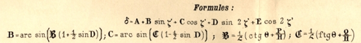
You can see that there is a mistake in the printed formulas on the chart—the terms in the inner parentheses in B and C should be divided, not multiplied. With D given as 6°45′, the value of ½ sin D is relatively small (about 0.06), and the error has a quite small effect on the overall result. It is not clear whether these incorrect formulas were used in designing the chart or whether they are due to an error on the part of the letterer or printer. As I will discuss a bit later, I performed quite a few tests of the accuracy of this chart based on a model of the Earth’s magnetic field at that time; from those tests it appears that the chart design itself was based on the incorrect formulas, but the differences in the results are small and the inherent inaccuracies in the chart and model make the distinction difficult.

Using Lallemand’s Chart

Directions for the use of the L’Abaque Triomphe are provided along the bottom of the chart, and there is even an example in dashed lines worked out on the chart itself.

Let’s follow the dashed line example marked on the chart highlighted in the figure below. The ship Le Triomphe is located at latitude 42°N and longitude 20°W and has a compass heading (or compass course) of 41.5° (read clockwise from North).

---

Step 1: The navigator locates the lat/long point on the map along the left side, moves from this position horizontally to the radial line pointing to the 41.5° course along the top, and marks this point.

Step 2: The same lat/long position is found in the upper map on the right side and followed along the guide lines to the line pointing again to the 41.5° course along the edge, marking that point.

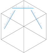
Step 3: A transparent or translucent overlay about the size of the paper and marked with a hexagon as shown in lower right of the figure is aligned square to the page with two of its radial arms crossing the two marked points from Steps 1 and 2. The Appendix of this essay contains a printable hexagonal overlay for use with the charts in this essay.

Step 4: The course correction is read from intersection of the next hexagon arm and the deviation scale (11.8°).

---

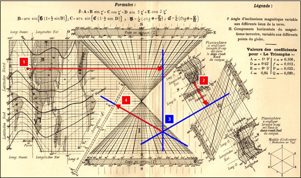
The compass course has this 11.8° deviation easterly from North, so the compass course has to be adjusted to obtain a true course of 41.5°. It surprises me that the correction for magnetic variation is not included in the result, as we will see that it was used in the calculation of the magnetic deviation.

If the compass course were southerly (90° to 270°), step 2 would be performed based on the lower map on the right side rather than the upper map.

The Accuracy of Lallemand’s Chart

So how accurate is it? The U.S. Geological Survey has modeled the magnetic variation around the world over the last few centuries. The figures below show the horizontal component and inclination (dip) of the Earth’s magnetic field in 1884, the year prior to the creation of the abaque. One microTesla is equivalent to 1/100 Gauss, so for example the horizontal intensity of the magnetic variation in Paris in 1884 was 19µT or 0.19G.

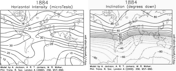
We can insert values from these figures at different locations on Earth into Lallemand’s equations and compare the result to that obtained graphically from the abaque. It is important to note that the prime meridian (0° longitude) is located at Paris in Lallemand’s chart; the French did not accept Greenwich as the prime meridian until 1911.

Also, there is no indication of the units of the “magnetic force” used in Lallemand’s chart, and any units could be used since the constants would scale any units appropriately; unfortunately, there are no units listed with these constants. Initially I presumed that H would be magnetic flux density in units of Gauss, since Maxwell and Thomson extended the cgs system of units with such electromagnetic units in 1874, but these units do not produce consistent results in the abaque. I later bought a copy of the Admiralty Manual for the Deviations of the Compass from 1893, in which Archibald Smith and F.J. Evans lay out the rationale for the equations used in Lallemand’s chart, and discovered that they normalized H to 1.0 at its value at Greenwich. We can assume that Lallemand normalized H to 1.0 at Paris instead (the difference is not large), so a horizontal intensity H from the 1884 USGS figure has to be multiplied by 1.0/0.19 = 5.26 before using that value in Lallemand’s formulas.

The results of my tests for various locations and courses are found below. The first row compares the computed value with the graphical value at the canonical location of 42°N 20°W. The rest of the rows are for different locations and/or different compass courses. The top spreadsheet compares the graphical results with computations based on the formulas listed on the chart, while the second spreadsheet uses the mathematically correct formulas for B and C.

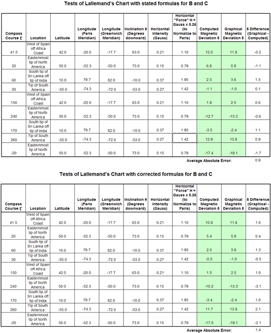
A lower average absolute error over the tested locations and compass courses is found in the top spreadsheet, suggesting that the chart was drawn using the incorrect formulas found on the chart, although the uncertainties in the graphical readings make this less than certain. In any event, the small difference between the two formulas is apparent.

The results are not bad at all given that we are estimating values off a model, certainly much, much better than not correcting for magnetic deviation at all. In addition, once you start taking measurements off the chart, you begin to notice that the abaque is a bit sketchy at places (look closely at the spacing of the vertical longitude lines in the map along the left side) and was most likely a proof-of-principle graphic.

How Does Lallemand’s Chart Work?

So how does it all work? Hexagonal charts in general are the subject of the next section of this essay, but at this point we state the conclusion: the hexagon arms point to three scales oriented 120° to each other and the value (offset) of the magnetic deviation scale δ is the sum of the values (offsets) of the other two scales. In the figure below the green lines cut the three scales at their zero points, and since these lines nearly intersect at the same point, then within some small error the hexagon will connect the zero values on the three scales (0+0=0). The values Y₁, Y₂ and Y₃ are the values (offsets) of the scales for the example of 42°N 20°W. With a ruler you can verify that Y₃ =Y₁ + Y₂ in length except for a small error (~1mm at the scale of the full-page version shown earlier) due to the inaccuracy in the chart as manifested by the inexact intersection of the green lines.

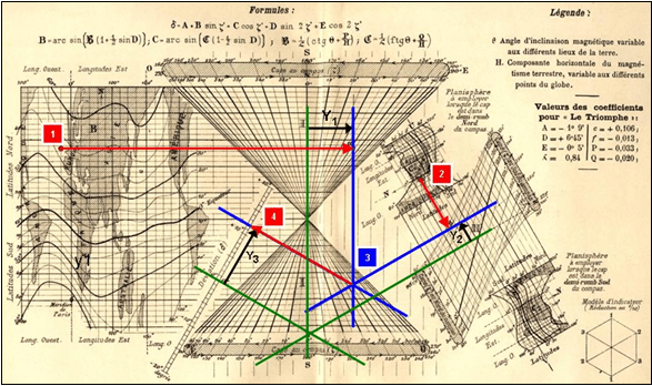
Let’s look at the construction of the three scales. Each represents an offset from an axis, and one of the advantages of this type of chart is that it doesn’t make any difference where along this axis this offset occurs. So in the first scale the offset Y₁ can occur anywhere along the vertical green x-axis of the scale, and this is true for Y₂ on the second scale. This allows the scales to be shifted anywhere along the green axes for optimum placement of the scales, and in fact it allows the Deviation (δ) scale to be tucked in the narrow space between the leftmost map and the central cone.

Now the leftmost map is drawn in such a way that the value of B for any latitude and longitude position provides a vertical offset B from the axis passing through the center of the cone. Extending this offset to the right provides a Y₁ value for the first term in the formula for magnetic deviation:

Y₁ = B sin ξ′

All of the other terms are combined into an offset generated from the maps on the right side of the chart :

Y₂ = A + C cos ξ′ + D cos 2ξ′ + E cos 2ξ′

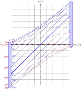To demonstrate the construction of the twisted cylindrical plot on the right side of the chart, I’ve plotted a graph here that shows Y₂ as a function of ξ′ for values of

• Latitude = 42°
• Longitude = 20° West (-20°)
• Inclination θ = +70° downward
• Horizontal H = 16 microTesla = .16 Gauss
• B = (1/.84)[0.106*tan θ + (-.033)/H)] = 0.101
• B = arcsin[B[1 + (sin(6.75°) / 2)]] = 6.15°
• C = (1/.84)[-.013*tan θ + (-.020)/H)] = 0.106
• C = arcsin[C[1 – (sin(6.75°) / 2)]] = 5.73°

Rotating this plot counterclockwise by 30° yields a y-axis that is 60° clockwise from the vertical axis of the chart, lying along the next arm of the hexagon. Note that the angles shown in this plot vary from 0° to 90° and 270° to 360°, which corresponds to compass courses ξ′ in northern half of the compass rose. The range ξ′ = 90° to 270° cross in the opposite direction, which is why there is a separate map used for compass courses ξ′ in the southern half of the compass rose. The offsets for the various latitude and longitude locations, using H and θ for the local magnetic variation, provides the curved lines on the lower and upper maps. This is where the enormous manual effort by Lallemand to create this chart is most apparent.

In the end the third arm of the hexagon overlay provides the sum of these two offsets, or

Y₃ = Y₁ + Y₂ = A + B sin ξ′ + C cos ξ′ + D cos 2ξ′ + E cos 2ξ′

which is the required equation for magnetic deviation.

Lallemands L’Abaque Triomphe is a uniquely interesting graphic because of the sophistication inherent in this first published hexagonal chart. No other chart of this type exists to my knowledge, although the use of hexagonal charts continued for some time until nomograms finally displaced them for good. The principles and history of hexagonal charts and their relatives, triangular coordinate systems, are the subject of Part II of this essay.

>>> Go to Part II of this essay

Highest Resolution and printer-friendly Word file of Lallemand’s L’Abaque Triomphe, Hexagonal Charts, and Triangular Coordinate Systems Parts I-II

Printer-friendly PDF file of Lallemand’s L’Abaque Triomphe, Hexagonal Charts, and Triangular Coordinate Systems Parts I-II