Dead Reckonings

William Thomson called them “beautiful and ingenious geometrical constructions,” and in variance to their rather humdrum name dygograms are certainly charming to the eye. But these geometric constructions can conveniently generate and then calculate the magnetic deviation of a ship compass at a location.

With our electronic calculators and computers, we take for granted the effortless arithmetic and trigonometric calculations that so vexed our ancestors. Pre-calculated tables for roots and circular functions, generated through hard work, were often used to create tables of magnetic deviations for specific ships and locations. To reduce the chance of misreading these tables, a few types of graphical diagrams, not just dygograms, were invented to provide fast and accurate readings of magnetic deviation. These graphical calculators are the focus of this part of the essay.

Computing the Magnetic Deviation

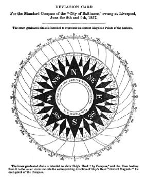
There were a few graphical methods of looking up the magnetic deviation on a ship at sea. A common type of chart, or deviation card, is shown in the figure on the right. Here the sailor would follow his compass heading on the inner circle and arrive at a course on the outer circle that is corrected for the magnetic deviation of the ship at the location for which the card was constructed.

A more typical chart invented in 1851 is called a Napier’s diagram after James Napier (1821-1879). The simple nature of this chart belies its advantages in obtaining a fast and reliable correction. To create it, vertical linear scales of compass courses are drawn (two for good resolution), along with with dotted and solid lines at 60° angles from the scales as shown in the figure (originally these were at 90° and 45°).
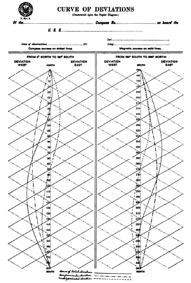Then the magnetic deviation is plotted opposite the scale, left (for west) or right (for east) such that the deviation for a given course is located on the solid line running 60° from the scale value. The semicircular and quadrantal components are also individually plotted as dashed curves in the ones I have seen. To read the correction, you would find the compass heading on the scale, proceed up the dotted line to the solid curve, then back to the scale along the solid line (or parallel to them for intermediate scale values). Then since the triangles are all equilateral, you’ve directly found the corrected compass heading without doing any arithmetic. Simple in design, robustly effective in use!

Napier’s diagrams could be directly plotted from data obtained as a ship was swung, and much was made of the then-new method of least squares in drawing the curves. It can be seen here that the solid curve is the sum of the plotted semicircular curve, the quadrantal curve, and the constant deviation A when significant. Only the semicircular deviation and the new total need to be re-plotted for other locations.

As ship design evolved from simple iron plating to iron hulls with larger engines, the inaccuracy of the inexact coefficients A, B, C, D and E became noticeable. On the other hand, the equation expressing the magnetic deviation in terms of the exact coefficients A, B, C, D and E was difficult to compute, despite a set of mathematical tables and rules specifically prepared for this purpose by Smith. In an attempt to deal with this, Smith invented the geometric constructions he called dygograms to provide a graphical calculation of the magnetic deviation for any compass course using the exact rather than inexact coefficients.

Dygograms

The Admiralty Manual for the Deviations of the Compass, by Smith and Evans, describes in detail two main types of dygograms, called Dygogram I and Dygogram II. We will briefly investigate each of these.

To create a dygogram for a given ship, it is assumed that the exact coefficients A, B, C, D and E are known. However, Smith does derive inverse series for extracting these exact coefficients from the inexact coefficients A, B, C, D and E that can be obtained by harmonic analysis from measurements taken as the ship is swung.

Dygogram I

Equation (2) in Part I of this essay expressed the magnetic deviation δ in terms of the inexact coefficients as reproduced below:

We see that the magnetic deviation consists of a constant value, semicircular terms with a period of 360°, and quadrantal terms with a period of 180°, each constant in magnitude. So as the ship swings completely around, the semicircular contribution make one revolution while the quadrantal contribution makes two revolutions. For the Dygogram I type, Smith modeled the net deviation as one point revolving on a circle at a certain angular speed, with a second point revolving on an outer circle centered on the first point but at half that speed. With correct scaling, the inner circle represents the contribution of the quandrantal terms while the outer circle represents the contribution of the semicircular components. An offset of A between the inner circle’s center and the origin completes the model.

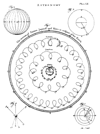This is an epicyclic motion similar to the Ptolemaic epicycles that modeled positions of the outer planets, except that Ptolomy had the outer circles rotating faster than the inner ones. This can also be modeled as a point on a circle as the circle rolls around the circumference of another circle, where here the effective radius of the inner circle is increased by the radius of the outer circle. This is akin to a penny rolling around another penny, in which Abraham Lincoln rotates twice for every revolution of the outer coin. Smith originally assigned the faster quadrantal rotation to the outer circle, and to me this is the instinctive way to do it, but by the 3rd edition of the Admiralty Manual he reversed these to take advantage of simplifications in construction proposed by Lieut. Colongue of the Russian Imperial Navy. It’s also a fact that the quadrantal force does not depend on the ship’s location, so he could affix this as the inner circle and then redraw only the outer curve for various locales.

The overall curve that results from a point rotating on a circle that is revolving around another point rotating on a circle is called The Limaçon of Pascal after its discoverer Étienne Pascal, father of Blase Pascal. It was named (from the Latin limax for snail) by Gilles-Personne Roberval in 1650 in his use of it to draw tangents as a means of differentiation. It has the general parametric form

          x = b cos θ + a cos 2θ

          y = b sin θ + a sin 2θ

or in polar coordinates,

          r = b + a cos θ

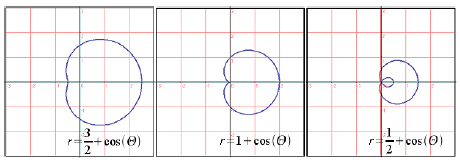
For a particular ship and location, the limaçon can be a circle if a = 0, it can approach but not touch the inner circle (as a dimpled circle) if a < b < 2a, it can just touch the inner circle (as a cusped curve, or a cardioid) if a = b, or it can loop within the inner circle and exit it if a > b. It’s a popular curve. As Smith describes it for p = b and q = a/2,

---

It is at once a conchoid of the circle, an epitrochoid, and a Cartesian oval. When p = q it gives, as was shown by Pascal, a solution of the problem of the trisection of the circle; when p = 2q it is a caustic by reflexion of the circle.

---

A Type I dygogram in high resolution from Lyons’ book can be seen by clicking here. We will be using miniature versions of it as we go. The dygogram calculates the magnetic deviation δ from the following equation in terms of the exact coefficients and the magnetic course ξ:

Now when the magnetic course is due north, we have ξ = 0° and the formula reduces to:

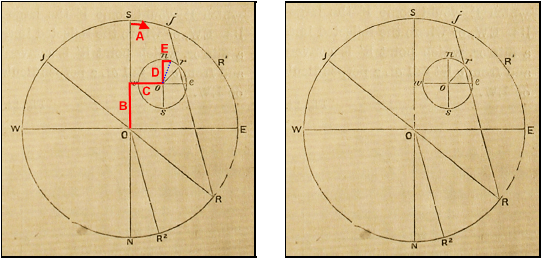
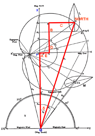Referring to the dygogram components in red in the figure to the right, we place a point O at the bottom of the page and at a convenient distance above it we place a point P. This distance is defined as the length of 1 in the dygogram and represents the mean directive force to north λH. Then using this as a unit length we move right a distance A to plot the point A, right again a distance E to plot the point E, up a distance D to plot the point D, up again a distance B to plot the point B, and right a distance C to plot the point C. From the figure you can see that Equation (4) for tan δ with ξ = 0° holds for this diagram, and therefore if magnetic north lies along the vertical line from O, that the angle from it to C (which is marked NORTH here) is the magnetic deviation when the ship is pointing north. So we mark this point C as N for the north magnetic course ξ = 0° and for clarity draw a ship pointing north at this point.

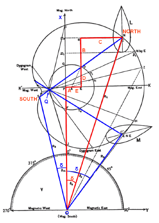
Now consider the blue markings we’ve added to our dygogram figure below on the left. For a magnetic course of due south, ξ = 180°, and from Equation (3) the only effect is that B and C, the distances that define the outer curve, change sign. So we extend (the math term is produce) ND a distance equal to ND in an opposite direction from point D and we get the appropriate point S (SOUTH) on the curve that will provide at O the magnetic deviation for a magnetic course of due south, that is, the angle between the vertical line OX and the line OS.

Now from the order in which we have placed these coefficients horizontally and vertically on the diagram you can see that the radius of the inner circle AD equals the magnitude of the sum of the quadrantal terms, or (D² + E²)^1/2. The distance DC equals the magnitude of the sum of the quadrantal terms, or (B² + C²)^1/2. The distance A simply produces a constant offset angle.

So let the magnetic course ξ proceed clockwise around from the north point N. If we rotate the constant radius AD by 2ξ about the point A while we rotate the constant distance DC by ξ around D, then the horizontal distance from the vertical line OX of the point on the curve will equal A + B sin ξ + C cos ξ + D sin 2ξ + E cos 2ξ while the vertical distance above O will equal 1 + B cos ξ + C sin ξ + D cos 2ξ + E sin 2ξ. Therefore, the tangent of the angle at O will be the ratio of these, and by Equation (3) the angle at O between the vertical line and the line to the point on the curve is the magnetic deviation δ for that magnetic course.

A limaçon is the curve that results from these required relationships. We mark a point Q where the north-south line NS intersects the inner circle. As the angle ξ rotates about Q, the segment DC will rotate at the same rate but the angle DAE will rotate at twice the angle. The point Q is called the pole of the dygogram and ξ is measured clockwise about it from QN. You can see on the figure that east-northeast is marked at a position 67.5° clockwise from N.

We construct the outer curve by laying a straightedge along NS and marking the positions of N, D and S on it, where D will be the midpoint of NS. We always need DC=DN to be a constant length from D, so we place the straightedge at various locations with D lying on the inner circle and passing through Q. At each location we mark points on the paper corresponding to N and S on the straightedge and we connect them to construct the curve. Then with a protractor centered at Q we mark various cardinal and intercardinal points of the compass on the outer curve and the dygogram is complete. The outer curve can indeed loop within the inner circle in some cases, as seen in the dygogram at the top of this essay which is also reproduced on the right. In practice most of the construction lines are removed in the final dygogram. From this graphical calculator we can now easily find the magnetic deviation for any magnetic course of the ship.

But again we would like to have the deviation in terms of the compass course ξ′ that we are reading on the ship. We know that δ = ξ ­– ξ′, so we can calculate from the dygogram the deviation for a given magnetic course and find the compass course as ξ —  δ, so we have the compass course for that magnetic course, but finding the deviation from a known compass course would be a trial and error process. Smith recommends laying out a Napier’s diagram for all the deviations, plotted offset along the solid lines from the compass course scale, and then using that diagram for any desired compass course. Smith also provides a couple of constructions to approximate the magnetic course for a desired compass course. But the best construction he describes is again due to Lieut. Colongue.

To demonstrate how we can find the magnetic deviation from the compass course, let’s first work backwards from the sample dygogram we’ve been using. In the figure on the right, for a north magnetic course of ξ = 0° we can read a magnetic deviation δ = 18° on the protractor (the angle between the vertical line OX and the north position of the ship in the upper right). Since δ = ξ –­ ξ′ we find that ξ′ = -18°. Now what we are going to do is to start with a compass course ξ′ = -18° and see if we end up calculating the same deviation δ = 18°.

The method is to first draw the (red) line from Q at the compass course angle ξ′ from the (green) line QN and mark the point where it intersects the vertical line OX. Then with dividers we draw the arc of a circle that passes through three points: O, Q and this intersection point. It will intersect the dygogram curve at the magnetic course ξ, and we proceed as before to find the deviation by the angle between OX and a line from O to that point. As you can see, it works out perfectly here, as that intersection corresponds to the north magnetic course that gave us δ = 18°. Using dividers to find the arc is analogous to trial and error, I suppose, but it’s a lot easier than doing math by trial and error, and this is one big advantage of graphical calculators in general.

Again, let’s verify it for the ENE location marked on the dygogram on the left. The magnetic course for this intercardinal point is 67.5° around Q from the north point N. We read from the protractor at the bottom that the deviation for this magnetic course is 36°, so we start with ξ′ = 67.5° — 36° = 31.5°. We draw a (red) line from Q at this angle from the (green) line QN and mark its intersection with OX. We draw the arc connecting O, Q and this point, and it indeed intersects the dygogram curve at the ENE point where ξ = 67.5°, from which we can read the deviation. So these two examples demonstrate that we can find the deviation for any compass course on the dygogram with a few extra steps.

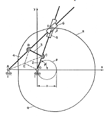Once the dygogram is constructed for one location, Smith provides simple procedures for plotting the dygogram at any other location from as few as two measurements of deviation vs. magnetic course at that place. In the process the values of the location-specific coefficients B and C are also found. Smith suggests a mechanical way of tracing the curve with a roller revolving about a roller in the same way as a coin revolves around the coin, but there are other ways to custom-draw a limaçon; I came across this mechanism in a book on linkages.

Dygogram II

Smith created an intermediate type of dygogram that consisted of an ellipse and a circle in lieu of the limaçon, but we are going to proceed to his ultimate form consisting of just two circles. I have only seen this discussed in the Admiralty Manual and in Smith’s obituary by Thomson, and only Thomson describes the case where A and E are non-zero. It is a clever transformation.

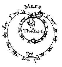Smith relates that it occurred to him to turn the paper with the same velocity that the ship turns, i.e., at the half-speed rotation of the outer generating circle, while tracing the limaçon in a same direction. Then the fixed point Q traces an inner circle, and the limaçon also ends up tracing another, outer circle. Here’s my guess as to how he might have come to that. Let’s zoom in on the innermost orbits in the figure of the Ptolemaic system we saw earlier. Here we see, from an Earth-centered point of view, the Sun revolving in a circular orbit around the Earth and Mars circling in what appears to be a perfect dygogram! And it very nearly is—it certainly is an epicycloid. If Mars were to have an orbital period of 2 Earth-years instead of 1.88 Earth-years it would be a dygogram, because the Sun point is modeled as revolving about the Earth with a period of 1 year and to match observations Mars must be modeled as revolving about the Sun point with a period of 2 years. Now as we know, Copernicus demonstrated that by changing the reference frame to a Sun-centered system (by fixing the paper on the Sun as the orbits trace) we find that the orbits of Earth and Mars end up as simple nested circles. We have an analogous situation here.

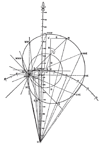
To construct this type of dygogram, a circle of radius 1 of some unit of length is drawn with a center O. Then using this unit length we move up from O a distance B and right a distance C and mark this point o. Then we move up a distance D and right a distance E. We draw a circle with its center at o that passes through this last point. This small circle is marked n, e, s and w and degrees are marked on it in a clockwise direction. The large circle is marked S, E, N and W but the position of these is rotated by A. Degrees are marked on it counterclockwise from north. Again Smith provides methods of plotting such a dygogram for different locations from a few observations. The finished dygogram appears as in the example below on the right.

Once the dygogram is created, Smith provides the following succinct procedure for reading the magnetic deviation for a given magnetic course:

---

Let ξ be the given magnetic course. Take R, a point on the circumference of the large circle, and r on the circumference of the small circle, such that NOR = nor = ξ, and join OR, Rr. Then ORr is the deviation which is +, or easterly, if r is to the right of O looking from R to O. If the large circle is graduated we may measure the angle ORr by producing RO, Rr, to intersect the circle in J and j. The arc Jj will then be twice the required angle.

---

But, again, on the ship we only know the compass course ξ′ we are reading from our compass. To use this we can place a straightedge that intersects the center O of the large circle and the value of ξ′ on the outer circle. Then we move it parallel to itself (there are linkages for parallel rulers) until it intersects the two circles at the same marked angle. These are the points R and r with values equal to the magnetic course ξ for this compass course, and we proceed from here as before to find the magnetic deviation. Again we see the power of a graphical calculator to naturally close in on a solution that would otherwise be a tedious trial-and-error arithmetic calculation.

Smith describes drawing a large set of lines between points on the two circles that have corresponding marked angles to provide a convenient, overall visual layout. Also, if the large circle is considered to be an upside down compass card, we can glue the (upside-down) small circle onto the compass card itself. In those days the needle was attached to the compass card, so the card turns with the needle and the compass course is the reading of the card in the forward direction the ship is facing. When the ship is at sea, we can find which drawn line between the two circles is fore-and-aft (which will be parallel to the compass course shown on the fore edge of the rotated card), and this will cut the two circles in points corresponding to the magnetic course. Or better yet, we can steer a magnetic course by turning the ship until the line connecting the desired magnetic course values on the two circles is fore-and-aft. Smith termed this a steering dygogram. It seems absolutely brilliant to me, but the lack of ready literature on it suggests it was never really taken up.

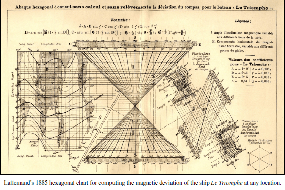
These graphical calculators—the Napier’s diagram and the various incarnations of the dygogram—are convenient devices for obtaining the magnetic deviation of a particular ship at a particular place. But a ship at sea would have to carry a set of charts like these for various locales, one more variable that could lead to disastrous errors. However, in 1885 a French engineer named Charles Lallemand created a uniquely designed and somewhat famous graphic, a hexagonal chart of his own invention, to calculate the magnetic deviation of the ship Le Triomphe no matter where it was located. The design and workings of this chart is the subject of another essay of mine, Lallemand’s L’Abaque Triomphe, Hexagonal Charts, and Triangular Coordinate Systems (under construction).

A Brief “Dygression”

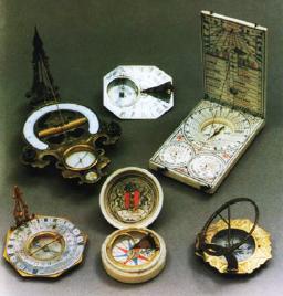In an article in 1907 A.G. Greenhill used a dygogram to model the reaction force on the axle of a pendulum. And just now as I write the final paragraphs of this essay, I look at the steering dygogram and it reminds me of sun compasses used as very early navigational aids. And that reminds me of portable sundials, which sparked my interest in nomography and graphical calculators in the first place. And that reminds me that the Equation of Time correction (the difference between the mean clock time and the actual solar time that must be accounted for in any good sundial) is composed of a sinusoidal term with a period of a year and a sinusoidal term with half that period!

Why this didn’t occur to me before is a mystery. During the few months I’ve been researching this essay, including reading through all the references and buying the only copy of Smith’s Admiralty Manual I could find in this hemisphere, I’ve also been plotting figure-8 analemma curves to represent the Equation of Time (EOT) correction on a sundial I’m designing for my house.

The non-circularity (or eccentricity) of the Earth’s orbit is one component of the EOT. The other component is the angle between the equator and the plane of the orbit (or the ecliptic tilt). Whitman provides a relatively simple but accurate formula for the EOT for a given day:

where Δt is the correction in minutes and (t — t₀) is the number of mean (clock time) solar days since the Earth’s perihelion (or closest approach to the sun).

The perihelion date varies with the year depending mostly on leap year differences, and it ranges from Jan. 3 to Jan. 5, so we can let t₀ = 4. The EOT is typically averaged over the four-year leap day cycle anyway. Then let α = 2π/365.24 and we have

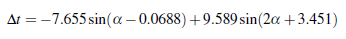
We can twice apply the identity

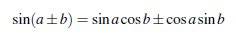
and find that

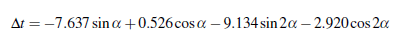
which is in the form of the magnetic deviation equation for the inexact coefficients A = 0, B = -7.637, C = 0.526, D = -9.134 and E = -2.920.

So a dygogram can model the EOT if the 365.24 days of the year are spaced out equally through the 360 degrees (about Q in Dygogram I and along the outer circle in Dygogram II). Now in an equatorial sundial the hour lines are also equally spaced around the circumference of a circle. So it might be possible to adapt the steering dygogram to provide the EOT correction right on the sundial. I will have to think about that.

An Exquisite Endeavor

The centuries it took to untangle the mysteries of magnetic deviation represent an enormous, sustained effort by scientists, mathematicians, ship captains and crews. Many people provided the mathematical and scientific tools and data needed to analyze the problem, and in fact this essay has focused only on contributors in the West. Captain Flinders, Edmund Halley, George Airy, William Scoresby, Archibald Smith and F. J. Evans sparked major advances in this area before gyrocompasses, ring gyros, and now LORAN and GPS diminished the importance of the compass. But it was so important then—a friend of his remarked that Smith was “penetrated by the conviction of the usefulness of his work.” Through his ténacité passionnée Smith produced a mathematical framework that defined magnetic deviation in a new and practical way, an achievement so beneficial that by the time he died, as Thomson relates,

---

From every ship in Her Majesty’s Navy, in whatever part of the world, a table of observed deviations of the compass, at least once a year is sent to the Admiralty, and is therefore subjected to [Smith’s] harmonic analysis.

---

From my point of view, the heroic efforts made by these men to overcome the deadly consequences of magnetic deviation comprise a very heartening thread of history and an inspiring illustration of the role of the mathematical sciences in advancing our civilization.

REFERENCES

The sources linked to Google Books are all fully viewable in the U.S., but not necessarily in other countries. If you find you are unable to read particular pages that you are interested in, please contact me and I will try to provide an excerpt for personal research under Fair Use provisions.

A Practical Manual of the Compass, A Short Treatise on the Errors of the Magnetic Compass, with the Methods Employed in the U.S. Navy for Compensating the Deviations and a Description of Service Instruments, Including the Gyro-Compass, The United States Naval Institute (1921), pp. 1-114. A collection of papers on the subject of magnetic deviation, measurement and corrections. It can be found here .

Barber, G.W, and Arrott, A.S. History and Magnetics of Compass Adjusting, IEEE Transactions on Magnetics, Vol. 24, No. 6, November, 1988. A refreshingly short and highly readable history of magnetic deviation.

Evans, F.J. Elementary Manual for the Deviations of the Compass in Iron Ships, 3rd Edition. London: J. D Potter (1875). As the title page says, this is “arranged in a series of questions and answers, intended for the use of Seamen, Adjusters of Compasses, and Navigation Schools, and as an introduction and companion to the Admiralty Manual for the Deviations of the Compass.” Worth reading to understand the basis of the deviation formulas, but oddly enough given his co-authorship of the Admiralty Manual, Evans does not treat dygograms at all. It can be found here.

Gibson, Lt. John. The Dygogram; Its Construction, Description and Use in Proceedings of the United States Naval Institute. United States Naval Institute (1984) pp. 555-571. A mathematically detailed article on the Type I dygogram, including a unique analysis of its validity by treating each magnetic component in isolation. It can be found here.

Grattan-Guinness, Ivor. The Search for Mathematical Roots, 1870-1940: Logics, Set Theories and the Foundations of Mathematics from Cantor through Russell to Gödel. Princeton University Press (2000). This is the source for the assertion that the first known appearance of the phrase harmonic analysis is in Thomson’s obituary of Archibald Smith, as cited by Jeff Miller at his website on Earliest Known Uses of Some of the Words of Mathematics (see harmonic analysis here). Thomson does say here that it is “commonly called” harmonic analysis, however.

Gray, Andrew. A Treatise on Magnetism and Electricity, Vol. I-II. Maps, Tables, Diagrams. New York: Macmillan (1898), Chap. IV, pp 85-100. Provides a derivation of Smith’s formulas for magnetic deviation, including the heeling error, and the construction of a Type I dygogram. It can be found here.

Greenhill, A.G. The Dygogram of Axle Reaction of a Pendulum, in Proceedings of the Edinburgh Mathematical Society, Vol. XXVI, 1907-1908, pp. 21-29 in second half of the volume. An interesting use of the dygogram to model other dynamic systems. Unfortunately, Figures 5 and 6 referenced in the article, which appear at the end of the volume, are only half-shown due to poor attention paid during scanning. It can be found here.

Gurney, Alan. Compass: A Story of Exploration and Innovation. New York: Norton (2005). A very entertaining, popular and surprisingly informative read on the history of the compass, including the effects and corrections due to magnetic deviation. Highly recommended!

Handbook of Magnetic Compass Adjustment. National Geospatial-Intelligence Agency (2004). A succinct and very clear summary of magnetic deviation, its effects on compasses, and sequenced steps to adjust compensators. It excludes the mathematical details of the derivations of the formulas and all graphical constructions.

Love, J.J. Review of Earth’s Magnetism in the Age of Sail (A.R.T. Jonkers, 2003). (2004). An interesting review and analysis of the history presented in the book (which I have not read). It can be found here.

Lyons, Timothy A. A Treatise on Electromagnetic Phenomena, and on the Compass and Its Deviations Aboard Ship: Mathematical, Theoretical, and Practical, Vol. II. J. Wiley & Sons (1903). An incredibly thorough account of the whole subject of compasses and magnetic deviation, including Type I dygograms and various means of correction. It can be found here.

Maor, Eli. Trigonometric Delights. Princeton University Press (1998). Chapter 7 of this book deals with epicycloids and hypocycloids. This is the source of the figure here of Ptolemy’s planetary scheme. The full book is available online here.

Muir, William C. P., A Treatise on Navigation and Nautical Astronomy: Including the Theory of Compass Deviations, Prepared for Use as a Text-book at the U. S. Naval Academy. United States Naval Institute (1906), pp. 55-203. A very good, comprehensive overview of the derivation of the formulas for magnetic deviation and Type I dygograms. It can be found here.

Smith, Archibald. Mr. Archibald Smith’s Introduction to Dr. Scoresby’s Journal of the Royal Charter, in The Magnetism of Ships and the Deviations of the Compass, Comprising the Three Reports of the Liverpool Compass Commission, Navy Department, Bureau of Navigation in Washington (1869). This volume if chock-full of detailed reports on magnetic deviation, but perhaps the one of most interest is the one on pp. 287-316 by Archibald Smith, in which he briefly describes the derivation of his formulas and refers to the long dispute between Airy and the then-deceased Scoresby over compass correction techniques, where Airy’s correction in fact did not work south of the (magnetic) equator. Smith attempts to be diplomatic, assigning most of the disagreement to a misunderstanding but allowing that “This mode of correction Dr. Scoresby, in common with many or most of those who examined the question, among whom I may rank myself, considered to be not only erroneous in principle but dangerous in practice.” I believe this is Smith’s introduction to Scoresby’s book that caused an immediate printed response by Airy that I read about. It can be found here.

Smith, Archibald. On the Mathematical Formulae Employed in the Computation, Reduction, and Discussion of the Deviations of the Compass, with Some Practical Deductions Therefrom as to the Mode of Construction of Iron-Built Vessels, in Transactions of the Institution of Naval Architects. Royal Institution of Naval Architects (1862), pp. 65-73. A relatively brief overview of the subject by Archibald Smith. It can be found here .

Thomson, William. Obituary Notices of Fellows Deceased in Proceedings of the Royal Society of London, Vol. XXII, from December 1, 1873 to June 18, 1874, pp. i-xxiv. A very nice, oft-referenced summary of the accomplishments of Archibald Smith in regard to magnetic deviation, including his derivations and dygogram construction, by his friend William Thomson (later Lord Kelvin). It can be found here. Note that this obituary is located nearly halfway through this two-volume book, not at the beginning as you would expect from the page numbers.

Whitman, Alan M. A Simple Expression for the Equation of Time. A relatively simple but accurate formula for a the Equation of Time is provided here, expressible as the sum of sinusoidal terms with the period of a year and the period of half a year in the same relationship as magnetic deviation. It can be found here.

<<< Go to Part I of this essay

Printer-friendly PDF of Magnetic Deviation Parts I-II